Download
1 / 30
300 likes | 429 Views
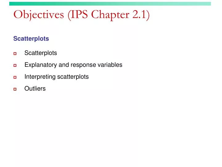
Objectives (IPS Chapter 2.1). Scatterplots Scatterplots Explanatory and response variables Interpreting scatterplots Outliers. Association between 2 variables. With 2 variables measured on the same individual , how could you describe the association ?

E N D
Objectives (IPS Chapter 2.1) Scatterplots • Scatterplots • Explanatory and response variables • Interpreting scatterplots • Outliers
Association between 2 variables • With 2 variables measured on the same individual, how could you describe the association? • Our descriptions will depend upon the types of variables (categorical or quantitative): • categorical vs. categorical - Examples? (smoke/lung cancer) • categorical vs. quantitative - Examples? (Gender/height), (City / Income of a group of people) • quantitative vs. quantitative - Examples? (Average working hours / Average GPA) • A scatterplot is the best graph for showing relationships between two quantitative variables
Association between 2 variables Here, we have two quantitative variables for each of 16 students. 1) How many beers they drank, and 2) Their blood alcohol level (BAC) We are interested in the relationship between the two variables: How is one affected by changes in the other one?
Association between 2 variables • One common task is to show that one variable can be used to explain variation in the other. • Explanatory variable vs. Response Variable Sometimes these are called independent(x) vs. dependent(y) variables. Eg: Here, we have two quantitative variables for each of 16 students. 1) How many beers they drank, and 2) Their blood alcohol level (BAC) But for some cases, it may be more reasonable to simply explore the relationship b/w two variables. Eg: High school math grades and high school English grades.
Association between 2 variables • These associations can be explored both graphically and numerically: • begin your analysis with graphics • find a pattern & look for deviations from the pattern • look for a mathematical model to describe the pattern • But again we do the above depending upon what type variables we have… we'll start with quantitative vs. quantitative ...
Scatterplots In a scatterplot, one axis is used to represent each of the variables, and the data are plotted as points on the graph.
Response (dependent) variable: blood alcohol content y x Explanatory (independent) variable: number of beers Explanatory and response variables A response variablemeasures or records an outcome of a study. An explanatory variableexplains changes in the response variable. Typically, the explanatory or independent variable is plotted on the x axis, and the response or dependent variable is plotted on the y axis.
Interpreting scatterplots • After plotting two variables on a scatterplot, we describe the relationship by examining the form,direction, and strength of the association. We look for an overall pattern … • Form: linear, curved, clusters, no pattern • Direction: positive, negative, no direction • Strength: how closely the points fit the “form” • … and deviations from that pattern. • Outliers
No relationship Nonlinear Form and direction of an association Linear
Positive association: High values of one variable tend to occur together with high values of the other variable. Negative association: High values of one variable tend to occur together with low values of the other variable. The scatterplots below show perfect linear associations
No relationship:X and Y vary independently. Knowing X tells you nothing about Y. One way to think about this is to remember the following: The equation for this line is y = 5. x is not involved.
Strength of the association The strength of the relationship between the two variables can be seen by how much variation, or scatter, there is around the main form. With a strong relationship, you can get a pretty good estimate of y if you know x. With a weak relationship, for any x you might get a wide range of y values.
Strength of the relationship or association ... This is a very strong relationship. The daily amount of gas consumed can be predicted quite accurately for a given temperature value. This is a weak relationship. For a particular state median household income, you can’t predict the state per capita income very well.
Outliers An outlier is a data value that has a very low probability of occurrence (i.e., it is unusual or unexpected). In a scatterplot, outliers are points that fall outside of the overall pattern of the relationship.
Objectives (IPS Chapter 2.2) CorrelationThe correlation coefficient “r” • r does not distinguish between x and y • r has no units of measurement • r ranges from -1 to +1
The correlation coefficient "r" • The correlation coefficient is a measure of the direction and strength of a linear relationship between two numerical variables. • r ranges from -1 to +1. • The sign of rgives the direction of a scatter plot. • |r| gives the strength of a scatter plot: • If |r| is close to 1, then the strength is strong. • If |r| is close to 0.5, then the strength is moderate. • If |r| is close to 0, then the strength is weak. • Note: if r=1, then it is perfect positive; if r=-1, then it is perfect negative.
Example to calculate “r” by hand • First, input all number into your calculator to get sample mean and sample SD for X and Y respectively. • Second, write out the formula one by one: • first get the product of each z-score of x and z-score of y, • then sum them up, • finally to divide it by (n-1).
Part of the calculation involves finding z, the standardized score we used when working with the normal distribution. You DON'T want to do this by hand. Make sure you learn how to use your calculator or software.
Example to calculate “r” by calculator • Input the data: Stat Edit Input X-values into L1; and input Y-values into L2. • Calculate correlation coefficient r: Stat Calc option 4. • If you can’t find r from your calculator, then you must follow the next slide to get the option of r back…
Subject: STT215: TI 83 / 84, where's the correlation coefficient?To find the correlation coefficient: • First, your calculator must be set up to display the correlation. (You only have to set it up once, so if you’ve done it in class, skip this part. Sometimes if you change batteries you have to do it again.) Hit 2nd CATALOG (this is over the 0 button). • Go down to DiagnosticOn, hit ENTER then ENTER again. It is now set up to display correlation with the regression line. 2. Enter the X values in one list and the Y values in another. Go to STAT>CALC 8:LinReg (a+bx) and hit ENTER. It is now pasted to the home screen. You must input the names of the list containing the X values followed by a comma then the list containing the Y values. For example, if my X values are in L1 and Y values are in L2, I would enter LinReg(a+bx) L1,L2 HWQ: 2.42 2.48 2.53 2.54
How do I restore deleted lists on a TI-83 family or TI-84 Plus family graphing calculator? • The instructions below detail how to restore deleted lists on a TI-83 family or TI-84 Plus family graphing calculator.To restore the original list names (L1 - L6):• Press [STAT]• Select 5:SetUpEditor • • Press [ENTER] (Done should appear on the screen) • The original lists, L1 - L6, should now appear when using [STAT] [ENTER]. • Please see the TI-83 family and TI-84 Plus family guidebooks for additional information.
Examples for correlation coefficient “r” Ex1. find the correlation coefficient of X and Y. Ex2. find the correlation coefficient of X and Z, where Z=2*X. Ex3. find the correlation coefficient of X and Z, where Z= -2*X. Ex4. find the correlation coefficient of X and Z, where Z= X+10. EX5. find the correlation coefficient of Y and X. EX6. find the correlation coefficient of U and V. Plot the scatter plots for EX2, EX3, EX4, and EX6 Now summarize all properties we obtain from these exercises. X Y 1 3 3 5 4 7 6 9 U V 1 0 0 1 2 1 1 2
Examples for correlation coefficient “r” U V 1 0 0 1 2 1 1 2 X Y 1 3 3 5 4 7 6 9 Ex1. find the correlation coefficient of X and Y. Ex2. find the correlation coefficient of X and Z, where Z=2*X. Ex3. find the correlation coefficient of X and Z, where Z= -2*X. Ex4. find the correlation coefficient of X and Z, where Z= X+10. EX5. find the correlation coefficient of Y and X. EX6. find the correlation coefficient of U and V. Plot the scatter plots for EX2, EX3, EX4, and EX6 EX2 scatter plot EX3 scatter plot EX4 scatter plot EX6 scatter plot
r = -0.75 r = -0.75 "Time to swim" is the explanatory variable here, and belongs on the x axis. However, in either plot r is the same (r=-0.75). “r” does not distinguish x & y The correlation coefficient, r, treats x and y symmetrically.
r = -0.75 z-score plot is the same for both plots r = -0.75 "r" has no unit Changing the units of variables does not change the correlation coefficient "r", because we get rid of all our units when we standardize (get z-scores).
Correlation estimation Estimate the correlation coefficient from the scatter plot R=0.393 R=0.861 R=0.778 r = -1 r = -0.95 r = -0.5 r = -0.25 r = -0.05 r = 0.05 r = 0.25 r = 0.5 r = 0.95 r = 1
Correlation Estimation Estimate the correlation coefficient from the scatter plot R= - 0.9 R= - 0.39 R= -1 R= -0.95 R= -0.5 R= -0.25 R= -0.05 R= - 0.951 R= 0.05 R= 0.25 R= 0.5 R= 0.95 R= 1
Correlation only describes linear relationships No matter how strong the association, r does not describe curved relationships. Note: You can sometimes transform a non-linear association to a linear form, for instance by taking the logarithm. You can then calculate a correlation using the transformed data.
Summary #1: • The correlation coefficient, r, is a numerical measure of the strength and directionof the linear relationship between two quantitative/numerical variables. • It is always a number between -1 and +1. Positive r positive association Negative r negative association • r=+1 implies a perfect positive relationship; points falling exactly on a straight line with positive slope • r=-1 implies a perfect negative relationship; points falling exactly on a straight line with negative slope • r~0 implies a very weaklinear relationship HWQ: 2.28, 2.29 2.18
Summary #2: • Correlation makes no distinction between explanatory & response variables – doesn’t matter which is which… • Both variables must be quantitative • r uses standardized values of the observations, so changing scales of one or the other or both of the variables doesn’t affect the value of r. • r measures the strength of the linear relationship between the two variables. It does not measure the strength of non-linear or curvilinear relationships, no matter how strong the relationship is… • r is not resistantto outliers – be careful about using r in the presence of outliers on either variable