Download
1 / 61
650 likes | 910 Views
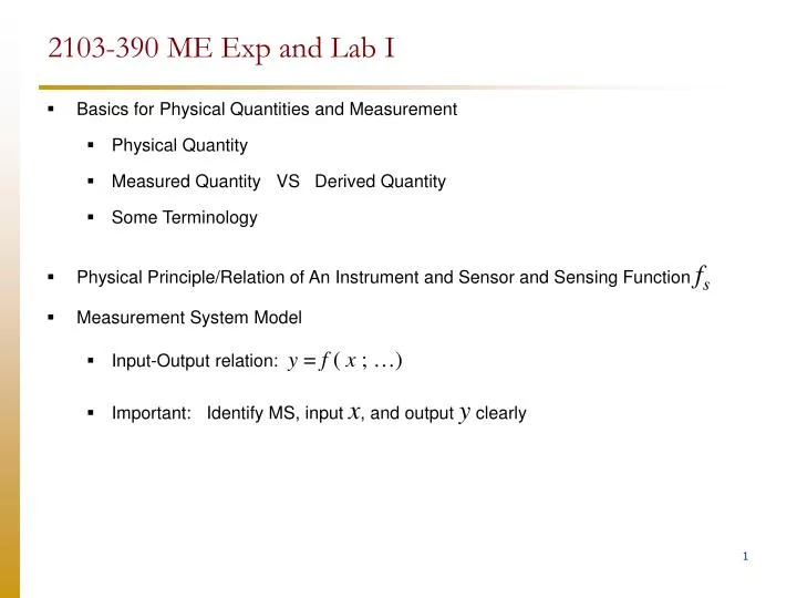
2103-390 ME Exp and Lab I. Basics for Physical Quantities and Measurement Physical Quantity Measured Quantity VS Derived Quantity Some Terminology Physical Principle/Relation of An Instrument and Sensor and Sensing Function f s Measurement System Model

E N D
2103-390 ME Exp and Lab I • Basics for Physical Quantities and Measurement • Physical Quantity • Measured Quantity VS Derived Quantity • Some Terminology • Physical Principle/Relation of An Instrument and Sensor and Sensing Function fs • Measurement System Model • Input-Output relation: y = f ( x ; …) • Important: Identify MS, input x, and output y clearly
Theoretical Input-Output Relation and Theoretical Sensitivity • Linear Instrument VS Non-Linear Instrument • Some Common Mechanical Measurements • Calibration • Static Calibration • Calibration Points and Calibration Curve • Calibration Process VS Measurement Process • Some Basic Instrument Parameters • Range and Span • Static Sensitivity K • Resolution • Some Common Practice in Indicating Instrument Errors
Describing a physical quantity q • Dimension • Numerical value with respect to the unit of measure • Unit of measure Physical QuantityDescribing A Physical Quantity Physical quantity • A quantifiable/measurable attribute we assign to a particular characteristic of nature that we observe.
Measured Quantity VS Derived Quantity The Determination of The Numerical Value of A Physical Quantity q must be either through • Measurement with an instrument Measured quantity or • Derived through a physical relation Derived quantity (and by no other means) Because of existing physical relations/laws, we don’t want anybody to make up any number for a physical quantity.
Some Terminology Measurement / Measure • The process of • quantifying, or • assigning a specific numerical value corresponding to a specific unit (of measure) to a physical quantity q of interest in a physical system. Measurand / Measured Variable • The physical quantity q that we want to measure, e.g., velocity, pressure, etc. Instrument / Measuring Instrument / Measurement System • The physical tool that we use for quantifying the measurand, e.g., thermometer, manometer, etc.
Often, our desired physical quantity x – measurand – cannot be measured directly (in its own dimension and unit). • Physical Principle/Relation of An Instrument ( fs ) • and • Sensor and Sensing Function fs
pb pressure at surface b Dh pa pressure at surface a rm Class Discussion What is the pressure difference (pa – pb)? Do we measure the pressure difference (pa – pb)directly in the unit of pa with a U-tube manometer?
pb pressure at surface b Dh pa pressure at surface a Dh (pa – pb) rm Input measurand x Measurement System (MS) y = fs ( x ; …) (sensor stage) Output y • What is the pressure difference (pa – pb)? • We do not measure (pa – pb) directly. • Instead, we measure Dh. • Then, determine the desired measurand (pa – pb) from the physical principle/relation (from static fluid)
Input measurand x Output y Dh (pa – pb) y Dh x (pa – pb) • Often, our desired physical quantity x – the measurand – cannot be measured directly (in its own dimension and unit). • We need to determine/derive its numerical value from • another physical quantity y, which is more easily measured, and • a physical relation/principle. Measurement System (MS) (sensor stage)
pb pressure at surface b Dh pa pressure at surface a rm Physical Principle/Relation of An Instrument [and Sensing Function fs] The physical principle of a U-tube manometer is static fluid (fluid in static equilibrium). • Physical Principle of An Instrument [and Sensing Function fs] • The physical principle that allows us to determine the desired measurand x with dimension [x] in terms of another physical quantity ys with different dimension [ys]. • We refer to the underlying physical relation as sensing functionfs.
pb pa Dh rm Principle: Fluid Static Dh (pa – pb) Input measurand x Measurement System (MS) Output y Physical Principle: Fluid Statics fsis the sensing function.
Sensor (or sensor-transducer) Output ys: ys = f (x;…) Measurement System / Instrument Process/System Signal Conditioning stage Output stage Sensor stage Transducer stage Signal path Input x Output y Control stage Thermometer Sensor/Transducer • employs physical phenomena • to sense the desired physical quantity x • in terms of another more easily measured quantity ys . Thermal expansion Temperature T Length L(scale)
Measurement System Model Input x Sensor stage (Sensing element) Signal Modification Stage Output Stage Output y (Numerical value ) Measurand q in a physical system f f s m Measurement System Model • Physical Principle of The Instrument and Sensing Function ( fs ) • We shall refer to • the physical principle that allows the sensor to sense the desired measurand x with dimension [x] in terms of another physical quantity yswith different dimension [ys] as the physical principle of the instrument, and • the corresponding underlying physical relation as the sensing functionfs.
Measurement System (MS) Input measurand x (physical quantity) Output y (physical quantity) • We are then interested inthe input-output relation Input - Output Relation: How to find the output-input relation - Theoretical - Actual Static Calibration
Input measurand x Measurement System (MS) Output y Important: Identify MS, input x, and output y clearly • When considering measurement system (or subsystem) characteristics • Measurement System: Identify the measurement system (MS) clearly (physically as well as functionally), from input x to output y. • Input Measurand x: Identify the physical quantity that is the input measurand x and its dimension/unit. • Output y: Identify the physical quantity that is the output y and its dimension/unit. • Calibration Curve: Find and draw the calibration curve ( y VS x ) for the system • Note: • It helps to identify the dimensions of the input and output physical quantities clearly. Is it length, pressure, velocity, or voltage, etc? • Recognize that if there is no output indicator, we cannot yet know the numerical value. • For example, the output of the pressure transducer is voltage output, but without a voltmeter or an output indicator, we cannot yet know the numerical value of this voltage output. • In this regard, e.g., when perform uncertainty analysis, the output indicator must be accounted for as part of the measurement system.
Measurement System Output Input First-Order System: Measurement System Model: First-Order System • The ODE has the solution where the complementary solution is given by and is the time constant. • The particular solution depends on the input forcing function.
= Normalized time 1/e = tn First-Order System: Step Forcing Input
Theoretical Input-Output Relation and Theoretical Sensitivity
pb pressure at surface b Define The Measurement System MS (Define the input and the output quantities clearly.) The Theoretical Input-Output Relation and Sensitivity Dh (output) Dh pa pressure at surface a pa –pb (input measurand) rm The input-output relation: Input measurand x ? Output y ? MS: U-Tube Manometer (pa –pb) [pressure] Dh [Length] The Theoretical Input-Output Relation and Theoretical Sensitivity forU-Tube Manometer
slope • Linear Instrument • Output y is a linear function of input measurand x. • The slope K is constant throughout the range • General Non-Linear Instrument • Output y is not a linear function of input measurand x. • The slope K is not constant throughout the range Theoretical Input-Output Relation and Graph, andLinear VS Non-Linear Instrument
Outputy Input measurandx Measurement System (MS) Sensitivity Sensitivity K • If K is large, small change in input produces large change in output. • The instrument can detect small change in input measurand more easily.
Example 1: Define MS, Input x, Output y Clearly Note: Here, we define a measurement system in a more general term, based on the interested functional relation.
+ + 2 1 rm= density of manometer fluid ra= density of fluid a rb= density of fluid b pa = static pressure at center a pb = static pressure at center b p1 = static pressure at 1 p2 = static pressure at 2 ha = elevation at center a hb = elevation at center b h1 = elevation at free surface 1 h2 = elevation at free surface 2 Dh = h2 – h1
Measurement System 1 (MS1) + + Input measurand x ? Input measurand x ? Output y ? Output y ? U-Tube Manometer U-Tube Manometer + + pa –pb [pressure] p1 –p2[pressure] Dh [Length] Dh [Length] Measurement System 2 (MS2) Example 1 Determine the theoretical input-output relations for the two measurement systems[See Appendix A for the derivation]
Example 2: Redefine our measurement system for convenience
+ + 2 1 Measurement System 1 (MS1) h [Length] Dh [Length] pa –pb [pressure] pa –pb [pressure] U-Tube Manometer U-Tube Manometer + + 2 Measurement System 2 (MS2) Equilibrium position 1 Example 2Redefine our measurement system for convenience • MS1: It is not convenient to measure the change from the two interfaces. • We may redefine our output/system. • MS2: Here, it is more convenient to measure the change with respect to one stationary reference point.
Example 3: Find the theoretical input-output relation and the theoretical sensitivity
+ + 2 (pa - pb) Dh Measurement System (MS) 1 The theoretical input-output relation is Example 3Find the theoretical input-output relation and the theoretical sensitivity
Example 4: Theoretical sensitivity and how to increase sensitivity in the design of an instrument
Example 4 How can we increase the sensitivity of the manometer?Differential Pressure Measurement - Inclined Manometer Principle: Static fluid Fox et al, 2010, Example Problem 3.2 pp. 59-61. • Appropriate sensitivity K can be chosen by changing d/D and sin q, e.g., • Smaller q Higher K
Some Common Mechanical Measurements • Temperature • Pressure • Velocity • Volume Flowrate • Displacement • Velocity • Acceleration • Force • Torque
Example 5: Differential Pressure MeasurementInclined Manometer Principle: Fluid Static From Dwyer http://www.dwyer-inst.com/PDF_files/Priced/424_cat.pdf
L = 0 L = 0 L (mmW) Input measurand x ? Output y ? Balance position: apply pa = pb Measure position: apply pa > pb Inclined Manometer Principle: Fluid Static pa –pb [pressure] (at the free surfaces) L [Length, mmW] From Dwyer http://www.dwyer-inst.com/PDF_files/Priced/424_cat.pdf
Example 6: Differential Pressure MeasurementPressure Transducer: Capacitance Principle: Capacitance From Omega: http://www.omega.com/ppt/pptsc.asp?ref=PX653&ttID=PX653&Nav=
Input measurand x ? Output y ? Pressure Transducer (alone) of the pressure transducer alone • Without output stage such as voltmeter or output indicator, however, we cannot yet know the numerical value of the output (voltage). • This is not yet a complete measurement system – no output stage. Pressure Transducer Principle: Capacitance pa –pb [pressure] (at the ports) V [Voltage, Vdc] From Omega: http://www.omega.com/ppt/pptsc.asp?ref=PX653&ttID=PX653&Nav=
Input measurand x ? Output y ? Pressure Transducer + Output Indicator • Specification/Characteristics (of the measurement system, e.g., accuracy, etc.) • Need to take into account the characteristics (e.g., accuracy, etc.) of the output stage – i.e., output indicator – also. Pressure Transducer + Output Indicator Principle: Capacitance pa –pb [pressure] (at the ports) V [Voltage, Vdc] From Omega: http://www.omega.com/ppt/pptsc.asp?ref=PX653&ttID=PX653&Nav=
Output Indicator (alone) From Omega http://www.omega.com/ppt/pptsc.asp?ref=DP24-E&Nav=
Calibration • Static Calibration • Calibration Points and Calibration Curve • Some Basic Instrument Parameters
CalibrationStatic Calibration Calibration is the act of applying a known/reference value of input to a measurement system. Objectives of Calibration Process • Determine the actual input-output relation of the instrument. • Quantify various performance parameters of the instrument, e.g., range, span, linearity, accuracy, etc. The known value used for the calibration is called the reference/standard. Static Calibration: • A calibration procedure in which the values of the variables involved remain constant. • That is, they do not change with time.
Calibration points: yM(x) Reference: Known value Static calibration curve (fit): yC(x) If it is linear, yC(x) = Kx + b. Calibration Points and Calibration Curve • Calibration Points: We first have a set of calibration points. • Calibration Curve: For convenience in usage, we fit the curve through calibration points and use the fitted equation in measurement.
Static calibration curve (fit): yC(x) Reference: Known value Reference: Known value Measurement process Calibration process Calibration Process VS Measurement Process
ymax ro =ymax - ymin ymin ri = xmax - xmin xmax xmin Some Basic Instrument ParametersRange and Span Calibration Range: Input range: Output range: Span: Input span: Output span: Full - scale operating range (FSO) = Output span =
Static calibration curve (fit): yC(x) If it is linear, yC(x) = Kx + b. Calibration points: yM(x) Some Basic Instrument ParametersStatic Sensitivity K Static Sensitivity: • is the slope of the static calibration curveyC(x)at that point. • In general, K = K(x). • If the calibration curve is linear, K = constant over the range.
Indicated output displays are finite/digit Continuous t Some Basic Instrument ParametersResolution (DRy) [Output] Resolution (DRy) is the smallest physically indicated output division that the instrument displays or is marked. Note that • while the input may be continuous (e.g., temperature in the room), • the indicated output displays are finite/digit (e.g., ‘digital’ or numbered scale on the output display). DRy
Output Resolution: DRy Linear static calibration curve: yC(x) = Kx + b. Indicated output displays are finite/digit, the input resolution is correspondingly considered finite. Some Basic Instrument ParametersResolution and Static Sensitivity KThe smallest change in input that an instrument can indicate. DRx: Input Resolution
Some Common Practice in Indicating Instrument Errors • Error e in % FSO: • Error e in % Reading: • Error e in [unit output]/[unit input]: