Gourley , Jonathan J., Baxter E. Vieux, 2005: A Method for Evaluating

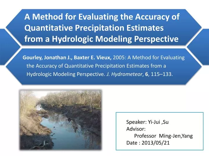
1. A Method for Evaluating the Accuracy of Quantitative Precipitation Estimates from aHydrologic Modeling Perspective Gourley, Jonathan J., Baxter E. Vieux, 2005: A Method for Evaluating the Accuracy of Quantitative Precipitation Estimates from a Hydrologic Modeling Perspective. J. Hydrometeor, 6, 115–133. Speaker: Yi-Jui ,Su Advisor: Professor Ming-Jen,Yang Date : 2013/05/21

2. Outline

3. introduction • The ensemble approach can provide a setting user-specified rangesand be more objective ∵it’s not a designed to favor a model input • The unique methodology has been developed to evaluate the relative skill of hydrologic simulations using different QPE inputs • Analyze the accuracy of the multisensor to QPE on hydrologic simulation

4. introduction Background • Blue River basin, Oklahoma • Hourly discharge observations from USGS KTLX(WSR-88D) (site number 07332500)

5. Methodology • QPE data • GAG (gauge only) • Oklahoma Meso-network(Mesonet) • 1km x 1km common grid using a Barnes scheme (Barnes 1964) • RAD (radar only) • Data from KTLX • Empirical formula :(Woodley et al. 1975) • MS (multisensor) • By QPESUMS (Gourley et al.2001) • Complex from radar, numerical models and infrared satellite data • Gauge-adjustmentfor RAD and MS 註1

6. Methodology Gauge-adjustment (Wilson and Brandes 1979) • Mean field bias adjustments (-G) • Local bias adjustment (-LG) (Seo and Breidenbach 2002) where ( βt is the threshold for multiplicative sample bias )

7. Methodology • Ranked probability score (RPS) • For the ensemble results, we use the Gaussian kernel density estimation to get the probability density function (pdf).(Silverman 1986) • To assess the ensemble skill, we use the ranked probability score(RPS; Wilks 1995) , where ↙ J is the event number

8. Methodology • Ranked probability score (RPS) Example: • If the threshold table of the pdfs as • the cumulative distribution function (cdf) + +

9. Methodology • Vlfo model (Vieux and Vieux 2002) • Bythe 1Dconservation of mass and momentum equations : • For the kinematic wave, the order of slope >> other forcing: , and we assume that it’s subcritical i :Soil infiltration rate r :Rainfall rate S0: bed slope Sf: friction slope • The Mannig’s equation in SI units: ; As w>>h ↖ R is the hydraulic radius • Substituting all into (B1), we got the governing equation used in the Vlfo model:

10. Methodology • Vlfo model(Vieux and Vieux 2002) Overland flow Channelized flow • The soil infiltration rate ( i ) use the Green-Ampt equation • To compute the cumulative infiltration (I), we should know K,ψand θ , and

11. Methodology • The variable inputted • n : Manning coefficient • r : rainfall rate • A: Cross-sectional area • Q : channel flow rate • S0: bed slope • K: saturated hydraulic conductivity • ψ: soil suction at wetting front (as 1/K ,Chow et al.1998) • θ: initial fractional water content

12. Work flow -G -LG 7 rainfall inputs 125 ensemble

13. Work flow The time of maximum discharge Compare to the observation • Runoff • coefficient • Bias • Mean absolute error • Root-mean-square error Mean value The maximum peak The total discharge volume

14. Results & discussion • Three case as follow • We just discuss the first case and its result

15. Results & discussion • Case1: 23 Oct 2002 • Total precipitation • -Gmaintain the pattern • -LGsmooththe spatial details • The KTLX radar was miscalibration and overestimate. (Gourleyet al.2003)

16. Case 1 MS MS RAD Time Peak RAD-G MS Discharge Volume

17. Case 1 • In the PDF pattern, Bimodal shape caused by the parameter maps set in the Vlfo model. • The members of θ set as 100% have higher peak and volume mode, but lower time density ∵ the nonlinear effect for the soil infiltration rate ↖ The infiltration as ponding

18. Case 1 Time Peak overestimate GAGRADRAD-GRAD-LGMSMS-GMS-LG GAGRADRAD-GRAD-LGMSMS-GMS-LG Volume overestimate GAGRADRAD-GRAD-LGMSMS-GMS-LG

19. Case 1 • RAD-G have the best performance in Time • The MS ,MS-G are bad predictions in Time, but good in Peak and Volume • Having more relationship with the gauge data(GAG,RAD-LG,MS-LG) will tend to have better performance in time than in peak and volume • -LG were bad in Peak and Volume

20. Summary and conclusions • Setting the range of parametric uncertainty andthe algorithms of objectively evaluating QPE provide more objective estimation. • θis a important parameter for infiltration, we need the initial data and the spatial variability. • Ranked probability score (RPS) can show the capability for ensemble forecast.

21. Summary and conclusions • Rain gauge data can’t provide a accurate depiction of the spatial variability of the rainfall field . • Satellite data may play an important role in QPE where ground-based radar cannot obtain a representative, low-level sample.

22. Summary and conclusions • Mean field bias adjustment(-G) have better result than local bias adjustment (-LG) in the hydrologic simulation. ∵ -LG emphasis on individual rain gauge measurements, and the spatial details in original rainfall field are smoothed. -G -LG 在雷達資料的空間分佈下做變化，但會因降雨分布跟雨量筒位置的關係而錯估降雨 保留相較於雨量計資料高估的估計，而低估部分則是雨量計的線性內差

23. References • Gourley, Jonathan J., Baxter E. Vieux, 2005: A Method for Evaluating the Accuracy of Quantitative Precipitation Estimates from a Hydrologic Modeling Perspective. J. Hydrometeor, 6, 115–133. • Wilks, D. S., 1995: Statistical Methods in the Atmospheric Sciences: An Introduction. Academic Press, 467 pp. • Seo, D.-J., and J. P. Breidenbach, 2002: Real-time correction of spatially nonuniform bias in radar rainfall data using rain gauge measurements. J. Hydrometeor., 3, 93–111. • Wilson, James W., Edward A. Brandes, 1979: Radar Measurement of Rainfall—A Summary. Bull. Amer. Meteor. Soc., 60, 1048–1058. • Oklahoma Water Survey : http://oklahomawatersurvey.org/?p=387 • The KTLX radar : http://weather.gladstonefamily.net/site/KTLX

24. Thanks for Your Attention