Download
1 / 55
560 likes | 739 Views
On Scaling Relations for Spiral Galaxies. Riccardo Giovanelli. Aug 2003. Menu of the Day. Scaling Relations for Spirals : from theory Scaling Relations : as observed Cosmology applications - briefly Kinematical scale length: extinction and inner disk M/L

E N D
On Scaling Relations for Spiral Galaxies Riccardo Giovanelli Aug 2003
Menu of the Day • Scaling Relations for Spirals : from theory • Scaling Relations : as observed • Cosmology applications - briefly • Kinematical scale length: extinction and inner disk M/L • Dwarf halos: are they really cuspy?
Disk Formation: a primer • Protogalaxies acquire angular momentum through tidal torques with nearest neighbors during the linear regime [Stromberg 1934; Hoyle 1949] • As self-gravity decouples the protogalaxy from the Hubble flow, [l/(d l/d t)]becomes v.large and the growth of l ceases • N-body simulations show that at turnaround time values of l range between 0.01 and 0.1, for halos of all masses • The average for halos isl = 0.05 • Only 10% of halos havel < 0.025 or l > 0.10 • halos achieve very modest rotational support The spin parameter l quantifies the degree of rotational support of a system : For E galaxies, l ~ 0.05 For S galaxies, l ~ 0.5 • Baryons collapse dissipatively within the potential well of their halo. They lose energy through radiative losses, largely conserving mass and angular momentum • Thus l of disks increases, as they shrink to the inner part of the halo. • [Fall & Efstathiou 1980] Angular momentum Mass Total Energy • If the galaxy retains all baryons m_d~1/10 , • and l_disk grows to ~ 0.5, R_disk ~ 1/10 R_h (mass of disk) /(total mass)
Scaling Laws for Disks * For starters, assume that halos are isothermal spheres, i.e. * Define as the limiting radius of the halo that which encloses a mean density equal to 200 times the critical density * Since * For standard choice of units:: where: [see Mo et al 1998; ; Dalcanton et al. 1997; Firmani & Avila-Reese 2000]
Scaling Laws for Disks then : * If the disk mass fraction is * If the disk mass assumes an exponential distribution * and if the disk angular momentum fraction is then
Scaling Laws for Disks When a more realistic density profile is adopted (e.g. NFW), the scaling relations of disks become: Where are dimensionless parameters of order 1, that take into account respectively the degree of concentration of the halo, the shape of the rotation curve and the radius at which it is measured.
… Assuming luminous and baryonic matter are similarly distributed in disks … …and introducing a disk mass to light ratio , we can convert disk mass surface density to surface brightness and disk mass to Luminosity, for comparison with observed scaling relations: 2 Note that theory predicts that b is proportional to l , c to l and a independent on l . Thus variance in halo l should affect differently the scatter in each relation.
… as for the observations… We use SFI++, a sample of 4000 spiral galaxies with I band accurate surface photometry; HI and/or Ha rotational data observed and processed by our group with the main purpose of mapping the cosmic peculiar velocity field.
Scale-length—Velocity Width • SFI and SFI+ samples: • I band CCD photometry • Sbc-Sc spirals • cz < 10000 km/s • HI and Ha spectroscopy • SFI : Giovanelli, Haynes, da Costa, • Freudling, Salzer, Wegner • 1600 galaxies • SFI++: Haynes & Giovanelli • 4000 galaxies
Central Disk Surface Brightness—Velocity Width Expected slope from Scaling law What about Freeman’s Law? [Freeman (1970)found that the central disk blue surface brightness is ~ constant for giant spirals] “Visibility” function
TF Relation: Data h= H/100 “Direct” slope is –7.6 “Inverse” slope is –7.8 SCI : cluster Sc sample …which is similar to the explicit theory-derived dependencea = 3 I band, 24 clusters, 782 galaxies [Giovanelli et al. 1997] a [WhereL a (rot. vel.) ]
TF Scatter Total error “Intrinsic” scatter Measurements + 0.30 mag Measurements + 0.25 mag Measurements + 0.20 mag Measurement error …measurement errors contribute the lesser part of the scatter
Cosmological Applications of the TF relation: • Measurement of the Hubble parameter • Assessment of the linearity of Hubble flow • Measurement of peculiar velocities: • - cosmic density field • - mass density parameter • - cluster and galaxy velocity dispersions • - cluster infall • - convergence depth of the local Universe • Evolution of M/L ratio with z
Convergence Depth Given a field of density fluctuations d(r) , an observer at r=0 will have a peculiar velocity: where W is W_mass The contribution to by fluctuations in the shell , asymptotically tends to zero as The cumulative by all fluctuations Within R thus exhibits the behavior : If the observer is the LG, the asymptotic matches the CMB dipole
The Dipole of the Peculiar Velocity Field The reflex motion of the LG, w.r.t. field galaxies in shells of progressively increasing radius, shows : convergence with the CMB dipole, both in amplitude and direction, near cz ~ 5000 km/s. [Giovanelli et al. 1998]
The Dipole of the Peculiar Velocity Field Convergence to the CMB dipole is confirmed by the LG motion w.r.t. a set of 79 clusters out to cz ~ 20,000 km/s [Giovanelli et al 1999 ; Dale et al. 1999]
1. Get good image of galaxy, measure PA, position slit So you want to measure a velocity width? 2. Pick spectral line, measure peak l along slit 3. Center kinematically 4. Fold about kinematical center 5. Correct for disk inclination, using isophotal ellipticity Outer slope 6. You now have a rotation curve. Pick a parametric model and fit it. E.g. Inner scale length
The rotation curve and the disk inclination combine to yield a set of isovelocity contours on the plane of the sky Disk opacity modifies V(r) A slit along the major axis yields a rotation curve … line of nodes pole-on … however, the l.o.s. may not penetrate all the way to the midplane of an inclined disk, effectively sampling regions in the foreground, off the disk major axis, as for an off-center slit, producing a shallower rotation curve.
On the Inner Scale length of V(r) With increasing disk opacity, the inner scale length of the observed V(r) should increase:: This effect had been investigated by comparing rotation curves observed in the same galaxy at very different l , thus affected differently by opacity, e.g. 21 cm and Ha. Increasing inner scale length For galaxies of given luminosity class, increasing disk inclination increasing l.o.s. opacity Thus we query: for a given class, does the inner scale length increase with disk inclination?
On the Inner Scale length of V(r) It does. More so for luminous than for intrinsically faint galaxies. Reason: column density and metallicity. Giovanelli & Haynes (2002, ApJL)
Modelling Extinction…. Valotto & Giovanelli (2003) The change of the inner scale length of V(r) with disk inclination can be modelled assuming that dust and stars have similar exponential distributions in both r and z. The observations (in this case for the brightest galaxies: M<-22) can be reproduced by a population with a scale height/scale length =0.145 and at l = 0.65 mm
On the Inner Scale length of V(r) Moreover note: at low inclinations, the mean inner scale length of V(r) appears to be the same for all galaxies
On the Inner Scale length of V(r) If we define f_d as (Disk Mass)/(Halo Mass) : Constancy of r_pe implies that, within that radius: i.e. baryonic contribution (disk + bulge) to M(r_pe) increases with galaxy mass . Nothing new here (Broeils 1992; Moriondo Giovanardi & Hunt 1998; Sellwood 1999) However : • Over range of 100 in halo mass of normal spirals, f_d within r_pe changes by ~ 5 • Most luminous spirals would have M(r) • fully baryon-dominated within inner few kpc • - then inner part of their rotation curves should scale • ~ like that of a pure disk for which (1-1/e)V_max • is reached at 0.63 disk scale lengths. M – 5 log(h) r_pe/r_d <-22 0.63 -21.7 0.68 -21.2 0.83 -20.7 0.95 -20.0 1.02 -19.0 1.28 Does it ? Use I – band images to measure r_d
On the Inner Scale length of V(r) We can then use rotation curves and I-band photometry to estimate the mean baryonic mass--to-light ratio of the inner region of bright spirals : Disk 1.6+/-0.7 Bulge 6.8+/-1.0 Which translates to a mean baryonic mass-to-bolometric light ratio of By measuring stellar velocity dispersions in NGC 7331, Bottema (1999) obtains
About Cusps of DM halos N-body simulations within the CDM scenario suggest a density profile for all halos of the form [Navarro, Frenk & White 1997]: Note: for small r for large r where the radial and the density scale parameters are related as The family of NFW density profiles can be parameterized via a halo concentration index
About Cusps of DM halos …are CDM halos too centrally cusped ? • The standard CDM structure formation scenario has been shown • to produce strongly cusped galaxy halos : with a=1 • Many observations suggest “softer” halo cores of nearly constant • density : a<0.5 [deBlok & McGaugh 1997; deBlok & Bosma 2002; • Marchesini et al. 2002; Swaters et al. 2002] • Simulations also produce halos with an unrealistic amount of • substructure (“halos within halos”) • …revised CDM versions within the framework of “concordance • cosmology” ( W_L=0.7, W_mass=0.3, h=0.7) appear to be able to • attenuate the conflict (Eke et al 20001)
About Cusps of DM halos [Spekkens & Giovanelli, in preparation] - Select a sample of dwarfs from SFI++, - Invert Poisson’s Eqn. and fit a line to the inner part of log r(r) to obtain a - We get, as most groups, values of a averaging about 0.5 - However, when we statistically fold in the observational biases (slit offset, misalignment, seeing, turbulent motions), we find that the derived values of a are compatible with a population with a=1
Inner Halo Structure from Direct Inversion Kristine Spekkens, Riccardo Giovanelli (Cornell) • Select 110 dwarf galaxies with Ha rotation curves, I-band photometry: no bulges, bars, interactions • Assume spherical matter distribution: density profile derived directly from RC. • Fit for the inner slope aof the density profile, and simulate expected distribution from population of CDM halos: Inner slopes are consistent with CDM halo cusps
Conclusions • Disk scaling relations are moderately well understood within the framework of hierarchical galaxy formation • Disk scale and surface brightness relations with rotational V are noisy and of limited utility (largely because of zero-point dependence on l : silver lining ) • After extinction effects are taken into account, the inner scale length of the rotation curve of spirals has a mean value that is independent on luminosity class. This indicates that the inner parts of bright spirals are baryon dominated, yielding a baryonic mass—to-light ratio of 1.9 • The observed Halpha rotation curves of dwarf galaxies are consistent with NFW halo density profiles ( r a 1/r ) • Most of the scatter of the TF relation is related to a galaxy’s formation history, rather than to observational errors • A template TF relation at low z can be determined with an accuracy of better than 0.03 mag, and profitably used to measure the rate and deviations of the Hubble flow in the local Universe, as well as other cosmological parameters • At high z, the TF relation is better suited to investigate the evolutionary history of disks
TF Relation: Data h= H/100 “Direct” slope is –7.6 “Inverse” slope is –7.8 SCI : cluster Sc sample …which is similar to the explicit theory-derived dependencea = 3 I band, 24 clusters, 782 galaxies [Giovanelli et al. 1997] a [WhereL a (rot. vel.) ]
Verrazzano Bias Pacific Ocean Map by Gerolamo da Verrazzano (1529)
On the Inner Scale length of V(r) - 3 What does the near constancy of r_pe mean? Mean density within r_pe Consider Radius within which the mean density is 200 times the critical density Mass within r_pe total mass at r_200 and, by definition, Since we get : and Since , a constant r_pe yields
Scale length and Central Disk Surface Brightness… …follow observed scaling relations with rotational velocity that are in agreement with theoretical predictions. However, these two parameters are not best suited for quantitative tests, because they * are poorly determined observationally * are subject (especially SB) to severe observational bias * exhibit strong dependence of scatter on galaxy formation history … Freeman’s law is apparent only when giant disks are seen in blue light. This results mainly because : (1) of internal extinction (which flattens the photometric profile and depresses central SB); (2) of sample selection biases; (3) the intrinsic scatter in the SB scaling relation is large, thus obscuring trend.
On the Inner Scale length of V(r) - 4 (*) Can we explain if it is assumed that DM dominates M (r) at all radii ? Take a NFW DM halo : At small r : And if r_pe is constant: (**) Relns. (*) and (**) match only if the concentration index c increases with total mass. However, N-body simulations show the opposite : they show c to decrease with mass.
The Luminosity-Linewidth Relation In 1977, R.B. Tully and J.R. Fisher proposed a relation between Luminosity and line width as a means to determine redshift-independent distances to galaxies. It can be derived from the scaling relation Defining a disk mass-to-light ratio , we can write where:
TF Relation: Observed Properties • Observers present the relation as one between absolute mag. and linewidth. The slope depends mildly on the photometric band, increasing to the red. • A mild type dependence is observed; even S0 gals exhibit a TF relation, albeit of > scatter [Neistein et al 1999; Hinz et al. 2001] • Observationally, it is the best established among scaling relations for disks. • In a PCA, the TF relation is an edge-on view of the fundamental plane of disks. No meaningful third-parameter dependences found. • The average scatter of the relation is ~ 1/3 mag near I band; it increases towards the blue. • Scatter depends on line width, and is not fully due to measurement errors.
TF Relation: best color • The quality of the TF relation depends on the band used in a variety of ways: • (a) Extinction increases towards the blue • (b) Bulge light increases towards the red • (c) Disk definition and estimate of its inclination degrade rapidly redwards of 1 micron • Point (c) is most important and advises for use of R or I band photometry
Can Theory Reproduce the Observed TF Relation? -1 The observed TF slope is explicitly returned by the theoretical expectation which yields a = 3 . However, that expectation matches observations only in the measure in which thecombination of parameters that make is luminosity (rotational speed) independent.
Can Theory Reproduce the Observed TF Relation? -2 The disk mass-to-light ratio is observed to be [Broeils 1992] N-body, gas-dynamical simulations yield [Navarro 1998] Assuming that the redshift of disk assembly is not largely different across the observed range of TF parameters, neutrality of A requires that the disk mass fraction (e.g. the ability of halos to retain their baryons) increase significantly with luminosity.
Can Theory Reproduce the Observed TF Relation? -4 N-body, gas-dynamical simulations can reproduce the slope and the scatter of the observed TF reln. They have difficulties reproducing the observed “zero point” offset, which are alleviated in LCDM simulations. [Navarro & Steinmetz 2000; Saiz et al. 2001] Challenges for N-body+hydro : • make halos w/low concentration • Force baryons to settle slowly • thus forcing disks to assemble • relatively late
Can Theory Reproduce the Observed TF Relation? -3 Evolution of the Mass-to-light ratio [Steinmetz & Navarro 1999] Star Formation Rate (solar masses per year) Lookback time (Gyr)
Does Evolution Affect the TF Relation? Palomar Keck Palomar: Bershady, Haynes & Giovanelli Keck: Vogt et al.
Collaborators At Cornell: At Jerusalem: At Rome: Daniel Dale Martha Haynes Terry Herter Marco Scodeggio Nicole Vogt Avishai Dekel Yehuda Hoffman Idit Zehavi Enzo Branchini At Trieste: At Dartmouth: At NRAO: Stefano Borgani Gary Wegner Eduardo Hardy At Wisconsin: At U. de Chile: At ESO: Matthew Bershady Luiz Da Costa W. Freudling Luis Campusano
Measuring the Hubble Constant A TF template relation is derived independently on the value of H . It can be derived for, or averaged over, a large number of galaxies, regions or environments. When calibrators are included, the Hubble constant can be gauged over the volume sampled by the template. From a selected sample of Cepheid Calibrators (e.g. Ferrarese et al. 2000), Giovanelli et al. (1997) obtain H_not= 69+/-6 (km/s)/Mpc averaged over a volume of cz = 9500 km/s radius. The HST key-project team [Sakai et al 2000] gets 71+/-4+/-7
TF and the Peculiar Velocity Field • Given a TF template relation, the peculiar velocity of a galaxy can be derived from its offset Dm from that template, via • For a TF scatter of 0.35 mag, the error on the peculiar velocity of a single galaxy is typically (0.15-0.20) cz • For clusters, the error can be reduced by a factor , if N galaxies per cluster are observed
No local Hubble Bubble Zehavi et al. (1999) : Local Hubble bubble within cz = 7500 km/s ? Giovanelli et al. (1999) :No local Hubble Bubble to cz ~ 15000 km/s
The Peculiar Velocity Field to cz=6500 km/s SFI [Haynes et al 2000a,b] Peculiar Velocities in the LG reference frame
The Peculiar Velocity Field to cz=6500 km/s Peculiar Velocities in the CMB reference frame SFI [Haynes et al 2000a,b]
Cosmological Parameters from the Peculiar Velocity Field VELMOD analysis of SFI and PSCz yields a value of = 0.42+/-0.04 [Branchini et al. 2001] Analysis of the velocity correlation function yields: With the resultb = 0.44+/- 0.05 [Borgani et al. 2000]