Download
1 / 3
30 likes | 203 Views
Part I. 10/9 – 11/10 Interpolation and Finite difference Numerical integration. Integration of ordinary differential equations. Symplectic integrator. (Tow-point boundary value problem, Spectral method or Fourier series: optional. ) Part II. 11/13 – 12/11

E N D
Part I. 10/9 – 11/10 Interpolation and Finite difference Numerical integration. Integration of ordinary differential equations. Symplectic integrator. (Tow-point boundary value problem, Spectral method or Fourier series: optional. ) Part II. 11/13 – 12/11 Finite difference scheme for the hyperboric equation. Finite difference scheme for the elliptic equation. Introduction for numerical relativity. Formulation of the Einstein’s equations in 3+1 form. Computational physics mini-course
0. Introduction References: ‘A Friendly Introduction to Numerical Analysis’, Brian Bradie, (Pearson Prentice Hall) ‘Numerical Recipe’, Press et al. (Cambridge) ‘Numerical computation’, C.W. Ueberhuber, (Springer) Computer aided researches in physics. • Experiments / Observations – Data processing and data analysis including statistical analysis, data modeling (e.g. c2 –fit)…. e.g. SDSS, LIGO • Tool for theoretical study – Numerical approximations, Simulations, Quantitative predictions. Symbolic calculations (manipulation for long equations).
This course is an introduction for numerical analysis. So, what do we use? Hardware check list – CPU power enough? Memory ? Storage (HD space)? Example for the softwares for computational physics on PC or a server. Numerical computing – Fortran, C++, and other computer languages. Symbolic Computation – Mathematica, Maple, Maxima. Graphics software and plotter – Gnuplot, xmgrace, supermongo visualization – OpenDX, IDL, AVS Unified environment – Octave, MATLAB