Download
1 / 68
800 likes | 1.04k Views
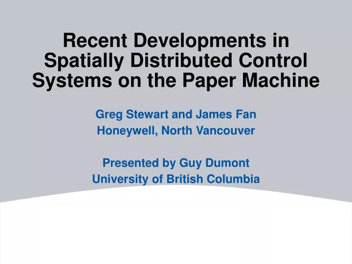
Recent Developments in Spatially Distributed Control Systems on the Paper Machine. Greg Stewart and James Fan Honeywell, North Vancouver Presented by Guy Dumont University of British Columbia. Outline. Industrial Paper Machine Operation Selected recent developments:

E N D
Recent Developments in Spatially Distributed Control Systems on the Paper Machine Greg Stewart and James Fan Honeywell, North Vancouver Presented by Guy Dumont University of British Columbia
Outline • Industrial Paper Machine Operation • Selected recent developments: • Automatic Tuning for Multiple Array Spatially Distributed Processes • Closed-Loop Identification of CD Controller Alignment
sheettravel Headbox and Table • Pulp stock is extruded on to a wire screen up to 11 metres wide and may travel faster than 100kph. Initially, the pulp stock is composed of about 99.5% water and 0.5% fibres.
suctionpresses Press Section • Newly-formed paper sheet is pressed and further de-watered.
Dryer Section finished reel • The pressed sheet is then dried to moisture specifications The paper machine picturedis 200 metres long and the paper sheet travels over 400 metres.
Dry End scanner • The finished paper sheet is wound up on the reel. The moisture content at the dry end is about 5%. It began as pulp stock composed of about 99.5% water.
Control Objectives • Properties of interest: • weight • moisture content • caliper (thickness of sheet) • coating & misc. • Regulation problem: to maintain paper properties as close to targets as possible. • Variance is a measure of the product quality.
weight moisture caliper MD CD Measurement gauges Paper Machine Process
Cross-Directional Profile Control • control objective: flat profilesin the cross-direction (CD) • a distributed array of actuators is used to access the cross-direction CD MD
Scanning Sensor • Paper properties are measured by a sensor traversing the full sheet width.
CD Actuator setpoint array, u(t) Sensor measurements MD Measured profile response, y(t) Cross-Directional Control
INPUT SIGNAL, u(t) LAN connection CONTROLLER, K(z) PROCESS, G(z) TARGET, r(t) LAN connection OUTPUT SIGNAL, y(t) Profile Control Loop
Supercalendering process • Supercalendering is often an off-machine process used in the production of high quality printing papers • The supercalendering objectives are to enhance paper surface properties such as gloss, caliper and smoothness • Typical end products are magazine paper, high end newsprint and label paper
Off Machine Supercalender Supercalenders • Gloss, caliper and smoothness are all affected by: • The lineal nip load • The sheet temperature • The sheet moisture content • With the induction heating actuators we can change the sheet temperature and the local nipload • With the steam showers we can change the sheet temperature and the sheet moisture content
Automatic Tuning for Multiple Array Spatially Distributed Processes
Automated Tuning Overview • Control problem • Multi-array cross-directional process models • Industrial model predictive controller configuration • Objectives of automated tuning • Two-dimensional frequency domain • Tuning procedure • Industrial software and examples • Conclusions
Multiple-array CD process models • Multiple-array process model:
Actuator setpoints CD Processes Sensor measurements LAN LAN (local area network) CD-MPC Controller LAN connected when needed Direct connection Real time QP solver Model identification Trial and error, Closed-loop simulations CD-MPC weights and closed-loop prediction Industrial MPC Configuration Automated MV Tuning Efficient and robust tuning
Objective function of CD MPC Prediction horizon Measurement weight Control horizon Aggressiveness penalty • The objective function • is minimized subject to actuator constraints • for optimal control solution Picketing penalty Energy penalty
Objectives of automated tuning • The tuning problem is to set the parameters of the MPC: • Prediction and control horizons (Hp, Hc) • Optimization weights (Q1, Q2, Q3, Q4) To provide good closed-loop performance with respect to model uncertainty (balance between performance and robustness) • Software tool requirements: • Computationally efficient implementation required for use in the field • Easy to use by the expected users
Automated Tuning Overview • Control problem • Multi-array cross-directional process models • Industrial model predictive controller configuration • Objectives of automated tuning • Two-dimensional frequency domain • Tuning procedure • Industrial software and examples • Conclusions
A 5-by-5 circulant matrices A 10-by-5 rectangular circulant matrices Circulant matrices and rectangular circulant matrices
Two-dimensional frequency • Based on the novel rectangular circulant matrices (RCMs) theory for CD processes,
Multiple-array plant model in the 2-D frequency domain • The model can be considered as rectangular circulant matrix blocks; and its 2-D frequency representation is
D(z) Y(z) Ysp U(z) + + + Kr K(z) G(z) _ Closed-loop transfer function matrices • Derive the closed-loop transfer functions of the system with unconstrained MPC. • Performance defined by sensitivity function • Robust Stability depended on control sensitivity function
Two-dimensional frequency bandwidth contour Sensitivity function for single array systems
(z) Robust Stability (RS) Condition • For additive unstructured uncertainty where is the representation of Tud(z) in the two -dimensional frequency domain. + + K(z) G(z)
Automated Tuning Overview • Control problem • Multi-array cross-directional process models • Industrial model predictive controller configuration • Objectives of automated tuning • Two-dimensional frequency domain • Tuning procedure • Industrial software and examples • Conclusions
Impact of MPC weights on Sensitivity Function1 • Interesting result: • MPC weight Q2 on u does not impact the spatial bandwidth • MPC weight Q4 does not impact the dynamical bandwidth • Encourages a separable approach to the tuning problem: 4.5 4 [cycles/metre] 3.5 Q4 3 n 2.5 2 1.5 i2 p w spatial frequency |t ( n ,e )<0.7071 yd Q2 1 0.5 -3 x 10 1 2 3 4 5 6 dynamical frequency w [cycles/second] 1 “Two-dimensional frequency analysis for unconstrained model predictive control of cross-directional processes”, Automatica, vol 40, no. 11, p. 1891-1903, 2004.
Tuning procedure Input plant info and knob positions Scaling Model preparation Horizon calculation Spatial tuning Dynamical tuning Results display Output tuning parameters
Automated Tuning Overview • Control problem • Multi-array cross-directional process models • Industrial model predictive controller configuration • Objectives of automated tuning • Two-dimensional frequency domain • Tuning procedure • Industrial software and examples • Conclusions
Example 1: linerboard paper machine (1) Four CD actuator arrays: u1 = Secondary slice lip; u2 = Primary slice lip; u3 = Steambox; u4 = Rewet shower; Two controlled sheet properties: y1 = Dry weight; y2 = Moisture; Overall model G(z) is a 984-by-220 transfer matrix. Performance comparison between traditional decentralized control and auto-tuned MPC.
Example 2: Supercalendars (1) Four CD actuator arrays: u1 = top steambox; u2 = top induction heating; u3 = bottom steambox; u4 = bottom induction heating; Three controlled sheet properties: y1 = caliper; y2 = top gloss; y3 = bottom gloss; Overall model G(z) is a 2880-by-190 transfer matrix. Performance comparison between traditional decentralized control, manually tuned MPC, and auto-tuned MPC.
Conclusions • A technique was presented for solving an industrial controller tuning problem – multi-array cross-directional model predictive control. • To be tractable the technique leverages spatially-invariant properties of the system. • Implemented in an industrial software tool. • Controller performance was demonstrated for two different processes.
Motivation • Uncertainty in alignment grows over time and can lead to degraded product and closed-loop unstable cross-directional control. • Typically due to sheet wander and/or shrinkage. Measured Bump response Actuator profile CD position [space]
Motivation • In many practical papermaking applications the alignment is sufficiently modeled by a simple function. • We assume it to be linear throughout this presentation.(Although the proposed technique is not restricted to linear alignment.) xj = f(j)
Current and Proposed Solutions
Solutions for Identification of Alignment Current Industrial Solutions: • Open-Loop Bumptest • Closed-Loop Probing Proposed Solution: • Closed-loop bumptest
Feedback diagram • The standard closed-loop control diagram. • r = target (bias target) • u = actuator setpoint profile • y = scanner measurement profile du dy + + r y u + + + G K -