Download
1 / 39
390 likes | 556 Views
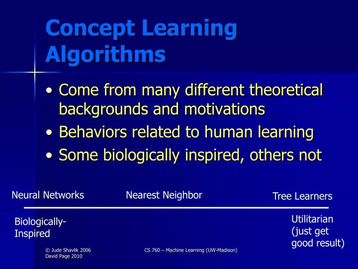
Concept Learning Algorithms. Come from many different theoretical backgrounds and motivations Behaviors related to human learning Some biologically inspired, others not. Neural Networks. Nearest Neighbor. Tree Learners. Utilitarian (just get good result). Biologically- Inspired.

E N D
Concept Learning Algorithms • Come from many different theoretical backgrounds and motivations • Behaviors related to human learning • Some biologically inspired, others not Neural Networks Nearest Neighbor Tree Learners Utilitarian (just get good result) Biologically- Inspired CS 760 – Machine Learning (UW-Madison)
Today’sTopics • Perceptrons • Artificial Neural Networks (ANNs) • Backpropagation • Weight Space CS 760 – Machine Learning (UW-Madison)
Connectionism PERCEPTRONS (Rosenblatt 1957) • among earliest work in machine learning • died out in 1960’s (Minsky & Papert book) wij J wik K I L wil Outputi = F(Wij * outputj + Wik * outputk + Wil * outputl ) CS 760 – Machine Learning (UW-Madison)
Perceptron as Classifier • Output for N example X is sign(W·X), where sign is -1 or +1 (or use threshold and 0,1) • Candidate Hypotheses: real-valued weight vectors • Training: Update W for each misclassified example X (target class t, predicted o) by: • Wi Wi + h(t-o)Xi • Here h is learning rate parameter CS 760 – Machine Learning (UW-Madison)
E ΔWj - η Wk E o (t – o) = (t – o) = -(t – o) Wk Wk Wk Gradient Descent for the Perceptron(Assume no threshold for now, and start with a common error measure) 2 Error ½ * ( t – o ) Network’s output Teacher’s answer (a constant wrt the weights) Remember: o = W·X CS 760 – Machine Learning (UW-Madison)
Continuation of Derivation (∑k wk * xk) E Stick in formula for output = -(t – o) Wk Wk = -(t – o) xk SoΔWk = η (t – o) xkThe Perceptron Rule Also known as the delta rule and other names (with small variations in calc.) CS 760 – Machine Learning (UW-Madison)
As it looks in your text (processing all data at once)… CS 760 – Machine Learning (UW-Madison)
W1X1 + W2X2 = Q X2 = = Q -W1X1 W2 -W1Q W2 W2 X1+ Linear Separability Consider a perceptron, its output is 1If W1X1+W2X2 + … + WnXn > Q 0otherwise In terms of feature space + + + + + + - + -- + + + + - + + -- - + + - - + - -- - - y = mx + b Hence, can only classify examples if a “line” (hyerplane) can separate them CS 760 – Machine Learning (UW-Madison)
Perceptron Convergence Theorem(Rosemblatt, 1957) Perceptron no Hidden Units Ifa set of examples is learnable, the perceptron training rule will eventually find the necessary weights However a perceptron can only learn/represent linearly separable dataset CS 760 – Machine Learning (UW-Madison)
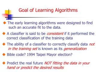
Output 0 1 1 0 a) b) c) d) Input 0 0 0 1 1 0 1 1 The (Infamous) XOR Problem Not linearly separable Exclusive OR (XOR) X1 1 b d a c X2 0 1 A NeuralNetwork Solution 1 1 X1 -1 -1 X2 Let Q = 0 for all nodes 1 1 CS 760 – Machine Learning (UW-Madison)
The Need for Hidden Units If there is one layer of enough hidden units (possibly 2N for Boolean functions), the input can be recoded (N = number of input units) This recoding allows any mapping to be represented (Minsky & Papert) Question:How to provide an error signal to the interior units? CS 760 – Machine Learning (UW-Madison)
A perceptron Hidden Units • One View • Allow a system to create its own internal representation – for which problem solving is easy CS 760 – Machine Learning (UW-Madison)
Advantages of Neural Networks Provide best predictive accuracy for some problems Being supplanted by SVM’s? Can represent a rich class of concepts Positive negative Positive Saturday: 40% chance of rain Sunday: 25% chance of rain CS 760 – Machine Learning (UW-Madison)
error weight Overview of ANNs Output units Recurrent link Hidden units Input units CS 760 – Machine Learning (UW-Madison)
Backpropagation CS 760 – Machine Learning (UW-Madison)
E Wi,j Backpropagation • Backpropagation involves a generalization of the perceptron rule • Rumelhart, Parker, and Le Cun (and Bryson & Ho, 1969), Werbos, 1974) independently developed (1985) a technique for determining how to adjust weights of interior (“hidden”) units • Derivation involves partial derivatives (hence, threshold function must be differentiable) error signal CS 760 – Machine Learning (UW-Madison)
Weight Space • Given a neural-network layout, the weights are free parameters that define a space • Each point in this Weight Spacespecifies a network • Associated with each point is an error rate, E, over the training data • Backprop performs gradient descent in weight space CS 760 – Machine Learning (UW-Madison)
E w Gradient Descent in Weight Space E W1 W1 W2 W2 CS 760 – Machine Learning (UW-Madison)
E wN E w0 E w1 E w2 , , , … … … , _ “delta” = change to w w The Gradient-Descent Rule E(w) [ ] The “gradient” This is a N+1 dimensional vector (i.e., the ‘slope’ in weight space) Since we want to reduce errors, we want to go “down hill” We’ll take a finite step in weight space: E E w = - E ( w ) or wi = - E wi W1 W2 CS 760 – Machine Learning (UW-Madison)
“On Line” vs. “Batch” Backprop • Technically, we should look at the error gradient for the entire training set, before taking a step in weight space (“batch” Backprop) • However, as presented, we take a step after each example (“on-line” Backprop) • Much faster convergence • Can reduce overfitting (since on-line Backprop is “noisy” gradient descent) CS 760 – Machine Learning (UW-Madison)
E w1 w1 w3 w2 w2 w3 wi w w w “On Line” vs. “Batch” BP (continued) * Note wi,BATCH wi, ON-LINE, for i > 1 BATCH – add w vectors for every training example, then ‘move’ in weight space. ON-LINE – “move” after each example (aka, stochastic gradient descent) E * Final locations in space need not be the same for BATCH and ON-LINE CS 760 – Machine Learning (UW-Madison)
outputi= F(Sweighti,j x outputj) Where F(inputi) = output j 1 1+e bias input -(inputi – biasi) Need Derivatives: Replace Step (Threshold) by Sigmoid Individual units CS 760 – Machine Learning (UW-Madison)
1 1 + e out i = - ( wj,i x outj) Differentiating the Logistic Function F(wgt’ed in) 1/2 F’(wgt’ed in) =out i( 1- out i) 0 Wj x outj CS 760 – Machine Learning (UW-Madison)
= (use equation 2) * See Table 4.2 in Mitchell for results = (use equation 3) Error Wi,j Error Wj,k wx,y = - (E / wx,y ) BP Calculations k j i Assume one layer of hidden units (std. topology) • Error ½ ( Teacheri – Outputi ) 2 • = ½ (Teacheri – F([Wi,j x Outputj] )2 • = ½ (Teacheri – F([Wi,j x F(Wj,k x Outputk)]))2 Determine recall CS 760 – Machine Learning (UW-Madison)
Derivation in Mitchell CS 760 – Machine Learning (UW-Madison)
Some Notation CS 760 – Machine Learning (UW-Madison)
By Chain Rule (since Wji influences rest of network only by its influence on Netj)… CS 760 – Machine Learning (UW-Madison)
Also remember this for later – We’ll call it -δj CS 760 – Machine Learning (UW-Madison)
Remember netk = wk1 xk1+ … + wkN xkN Remember that oj is xkj: output from j is input to k CS 760 – Machine Learning (UW-Madison)
outi = F( wi,j x outj) j Using BP to Train ANN’s • Initiate weights & bias to small random values (eg. in [-0.3, 0.3]) • Randomize order of training examples; for each do: • Propagate activity forward to output units k j i CS 760 – Machine Learning (UW-Madison)
F(neti) neti F’( netj ) = Using BP to Train ANN’s (continued) • Compute “deviation” for output units • Compute “deviation” for hidden units • Update weights i = F’( neti ) x (Teacheri-outi) j = F’( netj ) x ( wi,j x i) i • wi,j = x i x outj • wj,k = x j x outk CS 760 – Machine Learning (UW-Madison)
Using BP to Train ANN’s (continued) • Repeat until training-set error rate small enough (or until tuning-set error rate begins to rise – see later slide) Should use “early stopping” (i.e., minimize error on the tuning set; more details later) • Measure accuracy on test set to estimate generalization (future accuracy) CS 760 – Machine Learning (UW-Madison)
Advantages of Neural Networks • Universal representation (provided enough hidden units) • Less greedy than tree learners • In practice, good for problems with numeric inputs and can also handle numeric outputs • PHD: for many years, best protein secondary structure predictor CS 760 – Machine Learning (UW-Madison)
Disadvantages • Models not very comprehensible • Long training times • Very sensitive to number of hidden units… as a result, largely being supplanted by SVMs (SVMs take very different approach to getting non-linearity) CS 760 – Machine Learning (UW-Madison)
Looking Ahead • Perceptron rule can also be thought of as modifying weights on data points rather than features • Instead of process all data (batch) vs. one-at-a-time, could imagine processing 2 data points at a time, adjusting their relative weights based on their relative errors • This is what Platt’s SMO does (the SVM implementation in Weka) CS 760 – Machine Learning (UW-Madison)
Backup Slide to help with Derivative of Sigmoid CS 760 – Machine Learning (UW-Madison)