Download
1 / 38
380 likes | 554 Views
CORRELATIONS IN POLLUTANTS AND TOXICITIES. Kovanic P. and Ocelka T. The Institute of Public Health, Ostrava, Czech Republic. DATA. Actions: Regular monitoring of Czech and Moravian rivers Period: 2002 – 2007

E N D
CORRELATIONS IN POLLUTANTS AND TOXICITIES Kovanic P. and Ocelka T. The Institute of Public Health, Ostrava, Czech Republic
DATA • Actions: Regular monitoring of Czech and Moravian rivers • Period: 2002 – 2007 • Profiles: 21 locations of rivers Bečva, Berounka, Bílina, Dyje, Jihlava, Jizera, Labe, Lužická Nisa, Lužnice, Morava, Odra, Ohře, Opava, Otava, Sázava, Svratka, Vltava. • Field activity: Institute of Public Health, Ostrava (IPH) (The National Reference Laboratory) • Chemical analyses: Laboratories of the IPH, Frýdek-Místek • Mathematical (Gnostic) analysis: IPH • Particular problem: Are there any interactions between pollutants?
“NATURAL” ASSUMPTIONS ? • Contaminations are generated, polluted and accumulated mostly simultaneously, hence the more contaminants, the higher contamination and opposite. • The more pollutant A, the more polutant B. Positive and significant interactions between concentrations of pollutants are expected. IS IT TRUE?
COMMENTS • Concentrations of groups of pollutants differ by orders of magnitude. • Distributions differ not only by mean levels but also by their forms. • Distributions are non-Gaussian (“normal”): domains are finite, densities asymmetric. • Datavariability is strong, robust analysis must be applied.
TWO APPROACHES TO INTERACTIONS • Robust correlation coefficients: interdependence of deviations from the mean value • Robust regression models: interdependence of variables The former does not imply the latter automatically !
ROBUST CORRELATIONS • Robust estimate: low sensitivity to “bad” data • Non-robust estimates: point statistics (sample estimates of statistical moments) • Many robust estimates exist producing different results
DIVERSITY OF ESTIMATES • In the past: lack of robust methods • Recently: abundance of robust methods • Diversity of results: IN WHICH METHOD TO BELIEVE?
INFERENCE • Significant interactions between groups of pollutants have been confirmed. • Assumption of positive interactions was falsified: there exist negative interactions. • Group HCH initiates negative effects. • Interactions of groups implie interactions between individual congeners. Which congeners interact negatively and how much?
DEPENDENCE OF POLLUTANTS (“Y”) ON THE GAMMAHCH (“X”) Title L(Y)[L(X)]is to be read as ‘natural logarithm of the pollutant Y presented as a linear function of the natural logarithm of the pollutant X (gammaHCH)’ GRAPHS: Straight line is the robust linear model. Points depict the data values (X, Y) NOTE:Vertical scalings (of Y) differ, the horizontal scale (of X) remains unchanged
PARAMETERS OF THE FUNCTIONlognat(Y) = Intercept + Coef × lognat(gammaHCH) Pollutant (Y) Intercept STD(Intct) Coeff. STD(Coef) OCDD -1.01 0.23 -0.376 0.040 TCDD 0.080.34 -0.4240.057 PeCDD -0.94 0.28 -0.4540.048 HxCDD -2.580.16-0.0820.027 HpCDD -1.53 0.27 -0.3120.046 OCDF -1.55 0.28 -0.344 0.047 TCDF 2.01 0.35 -0.446 0.058 PeCDF 0.36 0.33 -0.319 0.055 HxCDF -1.58 0.27 -0.249 0.045 HpCDF -2.07 0.25 -0.184 0.041
PARAMETERS FOR THE HCH AND PBDE Pollutant (Y) Intercept STD(Intct) Coeff. STD(Coef) alfaHCH 2.14 0.38 0.373 0.064 betaHCH -2.39 0.57 1.054 0.096 deltaHCH -3.47 0.52 1.057 0.089 HCB 9.150.61-0.666 0.102 PBDE28 9.66 0.73 -1.603 0.123 PBDE47 15.30 0.69 -2.019 0.116 PBDE100 11.40 0.56 -1.698 0.095 PBDE99 13.39 0.71 -1.826 0.119 PBDE154 11.42 0.77 -2.004 0.130 PBDE153 9.92 0.71 -1.700 0.119 PBDE183 2.77 0.64 -0.534 0.105
RELATIVE IMPACTS OF gammaHCHImpact/mean(pollut.concentr.)(How many times is the mean exceeded)
POLLUTANT’S TOXICITY Four methods to measure toxicity: • Daphnia Magna • Vibrio Fischeri • Desmodemus subspicatus • Saprobita
“NATURAL” ASSUMPTIONS A) Methods measuring the same give thesame results or B) Results of measuring the same are at least similar (correlated) C) The more pollutant’s concentration, the more toxic effects
SIGNIFICANT CORRELATIONSWITH TOXICITIES Other correlations are not significant. “Natural” assumptions A) through C) are not supported by the data. Let us try the MD-models !
WORTHWHILE • MD-models confirm the existence of „contrary toxic effects“. • The group PCB affects the toxicity contrary to other groups of pollutants in3 of 4 MD-models in spite of the positiveness of all correlations (pollutant, toxicity).
SUMMARY Statistically significant (mostly positive) correlations in organic pollutants exist. Negative correlations exist as well. The most negatively “active” is gammaHCH. Its strongest negative effects are manifested by the congeners of PBDE. Contrary toxicity impacts of pollutants exist. HYPOTHESES MUST BE TESTED !
OPEN PROBLEMS Are these effects caused by some real chemical or physical reactions of the substances or only by different rates of their production and pollution? Are they worth of further investigation? EXPERIENCE: DATA TREATMENT MUST BE ROBUST AND HYPOTHESES MUST BE TESTED !
FUNDING European Commission Sixth Framework Program, Priority 6 (Global change and ecosystems), project 2-FUN (contract#036976)