Download
1 / 9
90 likes | 274 Views
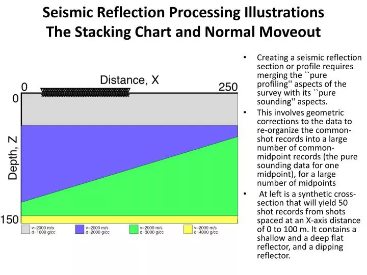
Seismic Reflection Processing Illustrations The Stacking Chart and Normal Moveout. Creating a seismic reflection section or profile requires merging the ``pure profiling'' aspects of the survey with its ``pure sounding'' aspects .

E N D
Seismic Reflection Processing IllustrationsThe Stacking Chart and Normal Moveout • Creating a seismic reflection section or profile requires merging the ``pure profiling'' aspects of the survey with its ``pure sounding'' aspects. • This involves geometric corrections to the data to re-organize the common-shot records into a large number of common-midpoint records (the pure sounding data for one midpoint), for a large number of midpoints • At left is a synthetic cross-section that will yield 50 shot records from shots spaced at an X-axis distance of 0 to 100 m. It contains a shallow and a deep flat reflector, and a dipping reflector.
The Stacking Chart and Normal Moveout • The pure profiling part of the reflection experiment is represented by the zero-offset time section at left. • Here the colors represent trace amplitudes, with cool colors for negative amplitudes and warm colors for positive. Green is zero amplitude. • This is the section that would result from towing a source and receiver together behind a boat, with no noise. The section simply uses the trace from each shot record with zero source-receiver offset, or distance. • By comparing with the model cross section above you can see (in time order) the shallow flat reflector, its surface multiple (note the surface reflection coefficient of -1), the dipping reflector, a second multiple of the shallow reflector, a surface multiple of the dipping reflector, and the deep flat reflector.
The Stacking Chart and Normal Moveout • Unfortunately, in land reflection work the zero-offset traces are the most contaminated by source-generated noise like air waves and surface waves, and the zero-offset section is useless. • The process of NMO correction, or stretching the seismograms in a CMP gather to flatten the hyperbolic reflection, together with stacking will emulate the zero-offset section and take advantage of the signal/noise enhancement provided by summing multiple traces over the fold.
The Stacking Chart and Normal Moveout Note the slight broadening of stacked pulses (NMO stretch), and the enhancement of flat reflections over multiples and dipping reflections.
The Stacking Chart and Normal Moveout • The data collected by a large number of pure sounding experiments along a profile forms a volume with 3 independent variables (xs, Xg, t), and the trace amplitude as the dependent variable. • Here large positive amplitudes are visualized as solids in warm colors, while small and negative amplitudes are made transparent. • The stacking chart above is on the top of the volume, and you can think of each seismogram as hanging from a point (xs, Xg) on the stacking chart. • On the right front face of this volume is a shot record in offset and time (Xg, t), showing the typical hyperbolic moveouts, and the direct arrival at the top. • Note that the dipping reflector actually has a negative moveout, from shooting it updip. • Of course this is just one shot record of many along parallel slices in the volume. This one is at (xs=100 m, Xg, t) with xs fixed at 100 m and Xg and t variable. • It is easy to figure our where each reflection is coming from by looking at the left front face of the volume. This perpendicular slice has variable shot location, offset fixed at zero, and variable time (xs, Xg=0, t). It is thus exactly the zero-offset section described above.
The Stacking Chart and Normal Moveout • At left, using our analysis of where the common midpoints lie on the stacking chart, we can simply slice the volume at the correct oblique angle (30 degrees for this survey) to obtain CMP gathers. The number of traces along each slice is its fold. Note that all reflections have hyperbolic normal moveout in the CMP gather, with their apexes at zero offset. This is true as well for the dipping reflector that had negative moveout in the shot record. The dipping reflector does show a higher apparent asymptotic velocity. • The slice at right is a CMP gather for a midpoint further to the right along the x axis. It is narrower and thus has a lower fold, and note that all contributions will be from longer-offset traces; there are no zero-offset traces for this midpoint.
The Stacking Chart and Normal Moveout • Here are the same CMP slices as the last slide, but we replaced the data volume with one in which the NMO-correction process has been carried out. This should work well, as the model section has constant and known velocity. • The hyperbolic moveouts have been removed, and all reflections have taken the time t0 of their hyperbolic apex. This is also the time of a flat reflector in the zero-offset section. • The slice at right is a CMP gather for a midpoint further to the right along the x axis. It is narrower and thus has a lower fold, and note that all contributions will be from longer-offset traces; there are no zero-offset traces for this midpoint. • Note that after NMO correction even the dipping reflector is flat across all traces, although only in the CMP slices. Note also the NMO stretch of the upper reflector at the farther offsets.
The Stacking Chart and Normal Moveout • Taking the NMO-corrected volume and viewing it level in the direction of stacking across the CMP fold shows what will happen in the stacked section. This view is similar to the stack above. • We look for structure in the zero-offset plane, and velocity in the shot gather. • As you look at the animation of the , try to trace the reflection surfaces and their geometry through the volume between the shot gather and zero-offset planes. • The purpose of the NMO correction is to subtract the additional time to a reflector due to increasing source-to-receiver offset, and bring the hyperbolic asymptotes level. After flattening, the volume can then be summed horizontally into the zero-offset plane, called stacking. • With real data this is the only way to see reflections on that plane, and why we have to perform profiling and sounding experiments concurrently in a real reflection survey.