Download

1 / 53
640 likes | 965 Views
Chapter 28 Weighted Graph Applications. Objectives. To represent weighted edges using adjacency matrices and priority queues (§28.2) To model weighted graphs using the WeightedGraph class that extends the AbstractGraph class (§28.3)

E N D
Objectives • To represent weighted edges using adjacency matrices and priority queues (§28.2) • To model weighted graphs using the WeightedGraph class that extends the AbstractGraph class (§28.3) • To design and implement the algorithm for finding a minimum spanning tree (MST) (§28.4) • To define the MST class that extends the Tree class (§28.4) • To design and implement the algorithm for finding single-source shortest paths (§28.5) • To define the ShortestPathTree class that extends the Tree class (§28.5) • To solve the weighted nine tail problem using the shortest path algorithm (§28.6)
Representing Weighted Graphs • Representing Weighted Edges: Edge Array • Weighted Adjacency Matrices • Priority Adjacency Lists
Representing Weighted Graphs • There are two types of weighted graphs • The vertices are assigned a weight • The edges are assigned a weight (what we are going to study) • Many applications
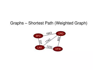
Weighted Edge Graphs • In a weighted graph, each edge has an associated numerical value, called the weight of the edge • Edge weights may represent distances, costs, etc. • Example: • In a flight route graph, the weight of an edge represents the distance in miles between the endpoint airports 849 PVD 1843 ORD 142 SFO 802 LGA 1205 1743 337 1387 HNL 2555 1099 1233 LAX 1120 DFW MIA
Representing Weighted Edges: Edge Array int[][] edges = {{0, 1, 7},{0, 3, 9}, {1, 0, 7},{1, 2, 9}, {1, 3, 7}, {2, 1, 9}, {2, 3, 7}, {2, 4, 7}, {3, 0, 9}, {3, 1, 7}, {3, 2, 7}, {3, 4, 9}, {4, 2, 7}, {4, 3, 9}}; vertex weight {0, 1, 7}
Representing Weighted Edges: Weighted Adjacency Matrices (1) • Assume that a graph has n vertices, one can use a n x n array to represent the weights • weights [i][j] represents the weight on edge (i,j) • If the vertices are not connected, then weights [i][j]= null • Weights do not have to be integers • Could be objects
Representing Weighted Edges: Weighted Adjacency Matrices (2) Integer[][] adjacencyMatrix = {{null, 7, null, 9, null }, {7, null, 9, 7, null }, {0, 9, null, 7, 7}, {9, 7, 7, null, 9}, {null, null, 7, 9, null}}; For example: (0,0) =null (0,1) = 7 (0,2) = null (0,3) = 9 (0,4)=null (1,2)=9 (2,4)=7
Weighted Graphs • Another way to represent edges is to define edges as objects • TheAbstractGraph.Edgeclass was defined previously to represent edges in un-weighted graphs (See Chapter 27) • For weighted graphs, we define the WeightedEdgeclass • To represents an edge from vertexuto v • WeightedEdgeextends AbstractGraph.Edgeto add the property weight • To create an Edge object • The Edge(i,j,w) object represents an edge where wis the weight on edge (i,j)
Priority Adjacency Lists (1) • Weight graphs using priority adjacency lists can be used to implement priority queues • Edges are removed in increasing order • Edge class implements the Comparable interface
Priority Adjacency Lists (2) • java.util.PriorityQueue<Edge> queues = new java.util.PriorityQueue<Edge>(); Note: weights are removed in priority order
The WeightedGraph Class Listings 28.1 -28.3 TestWeightedGraph TestWeightedGraph Graph AbstractGraph WeightedGraph
Trees and Forests • A (free) treeis an undirected graph T such that • T is connected • T has no cycles • A forestis an undirected graph without cycles • The connected components of a forest are trees Tree Forest
Spanning subgraph Subgraph of a graph G containing all the vertices of G Spanning tree Spanning subgraph that is itself a (free) tree Minimum spanning tree (MST) Spanning tree of a weighted graph with minimum total edge weight Applications Communications networks Transportation networks MST are not unique if the weights are not distinct Minimum Spanning Trees (MST) ORD 10 1 PIT DEN 6 7 9 3 DCA STL 4 5 8 2 DFW ATL
Minimum Spanning Trees Example • A cable TV company needs to lay cable to a new neighborhood • If it is constrained to bury the cable only along certain paths, then there would be a graph representing which points are connected by those paths • Some of those paths might be more expensive, because they are longer, or require the cable to be buried deeper; these paths would be represented by edges with larger weights • A spanning tree for that graph would be a subset of those paths that has no cycles but still connects to every house • There might be several spanning trees possible • A minimum spanning tree would be one with the lowest total cost
Minimum Spanning Trees • The trees in Figures 28.3(b), 28.3(c), 28.3(d) are spanning trees for the graph in Figure 28.3(a) • The trees in Figures 28.3(c) and 28.3(d) are minimum spanning trees 28.3(a) 28.3(b) (42) 28.3(c) (38) 28.3(d) (38)
Prim Minimum Spanning Tree Algorithm • The algorithm starts with a spanning tree T that contains an arbitrary vertex • The algorithm expands the tree T by adding a vertex with the smallest edge incident to the vertex already in T tree • (An edge that joins two vertices is said to be incident to both vertices)
Prim Minimum Spanning Tree Algorithm minimumSpanningTree() { Let V denote the set of vertices in the graph; Let T be a set for the vertices in the spanning tree; Initially, add the starting vertex to T; while (size of T < n) { find u in T and v in V – T with the smallest weight on the edge (u, v), (see Figure 28.4 on the next page) add v to T; } } Listing 28.4
Prim’s Minimum Spanning Tree Algorithm • The algorithm starts by adding the starting vertex into T • The algorithm continuously adds an adjacent vertex (v) from V - T with the smallest weight on the edge Figure 28.4
Prim’s Minimum Spanning Tree Algorithm 1 2 0 6 3 5 4
Adding Vertices using Prim’s Algorithm • Add vertex 0 to T • Add vertex 5 to T since edge (5,0,5) has the smallest weight (5) among the edges adjacent to T • Add vertex 1 to T since edge (1,0,6) has the smallest weight (6) among the edges adjacent to T • Add vertex 6 to T since edge (6,1,7) has the smallest weight (7) among the edges adjacent to T • Add vertex 2 to T since edge (2,6, 5) has the smallest weight (5) among the edges adjacent to T • Add vertex 4 to T since edge (4,6,7) has the smallest weight (7) among the edges adjacent to T • Add vertex 3 to T since edge (3,2,8) has the smallest weight (7) among the edges adjacent to T The adjacent vertices with the smallest weight are added successively
Minimum Spanning Tree Algorithm Example using Prim’s Algorithm
Implementing MST Algorithm The MST class extends the Tree class
Implementing MST Algorithm (1) • The getMinimumSpanningTree (int v) method is defined in the WeightedGraph class • It returns an instance of the MST class • The MST class is an inner class in the WeightedGraph class which extends the Tree class • The getMinimumSpanningTree (intstartingVertex) method first adds startingVertex to T • T is a set that stores the vertices currently in the spanning tree • Vertices is an array that stores all the vertices of the graph
Implementing MST Algorithm (2) • A vertex is added to T if it is adjacent to one of the vertices in T with the smallest weight • For each vertex is added to T, find its neighbor with the smallest weight to u • All the neighbors are stored in queues [u] • queues [u].peek() returns the adjacent edge with the smallest weight • If a neighbor is already in T, remove it • To keep the original queue intact, a copy is made
Time Complexity • For each vertex, the program constructs a priority queue for its adjacent edges • It takes O(log|V|) time to insert an edge to a priority queue and the same time to remove an edge from the priority queue • So the overall time complexity for the program is P(|E|log|v|) , where |E| denotes the number of edges and |V| denotes the number of vertices
Testing Minimum Spanning Tree (MST) Algorithm Listing 28.5 TestMinimumSpanningTree TestMinimumSpanningTree
0 A 4 8 2 8 2 3 7 1 B C D 3 9 5 8 2 5 E F Shortest Paths
Shortest Path • Section 27.1 introduced the problem of finding the shortest distance between two cities for the graph in Figure 27.1 • The answer to this problem is to find a shortest path between two vertices in the graph
Shortest Paths • Given a weighted graph and two vertices u and v, we want to find a path of minimum total weight between u and v • Length of a path is the sum of the weights of its edges • Example: • Shortest path between Providence and Honolulu • Applications • Internet packet routing • Flight reservations • Driving directions 849 PVD 1843 ORD 142 SFO 802 LGA 1205 1743 337 1387 HNL 2555 1099 1233 LAX 1120 DFW MIA
Dijkstra’s Algorithm (1) • The distance of a vertex v from a vertex s is the length of a shortest path between sand v • Dijkstra’s algorithm is used to find the shortest path • It computes the distances of all the vertices from a given start vertex s given the following assumptions: • The graph is connected • The edges are undirected • The edge weights are nonnegative
Dijkstra’s Algorithm (2) • The algorithm uses a costs[v] array to store the costs of the shortest path from vertex v to the source vertex s • costs[s]= 0 • Initially assign infinity to costs[v] to indicate that no path is found from v to s
Dijkstra’s Algorithm (3) • Let V denote all vertices and T denote the set of vertices whose costs have been found so far • Initially the source vertex s is in T • The algorithm repeatedly finds a vertex u in T and a vertex in V – T such that that costs[u] + w(u,v) is the smallest and moves v to T • w(u,v) denotes the weight of edge (u,v)
Dijkstra’s Single Source Shortest Path Algorithm shortestPath(s) { Let V denote the set of vertices in the graph; Let T be a set that contains the vertices whose path to s have been found; Initially T contains source vertex s; while (size of T < n) { find v in V – T with the smallest costs[u] + w(u, v) value among all u in T; add v to T; } } Listing 28.6
Single Source Shortest Path Algorithm (Dijkstra’s) • The algorithm starts by adding the source vertex s into T and sets costs[s] to 0 • It continually adds vertices,v to V – T into T • v is the vertex that is adjacent to a vertex in T with the smallest costs[u] + w(u,v) Finds a vertex u in T that connects a vertex v in V – T with the smallest costs[u] + w(u,v) There are five edges connecting vertices in T and V – T (u,v) has the smallest costs[u] + w(u,v) v will be added to T
Dijkstra’s Algorithm Example (1) • Suppose the source vertex is 1 • costs[1] = 0 • The costs for all other vertices are set to infinity - The algorithm will find the shortest paths from source vertex 1
Dijkstra’s Algorithm Example (2) • Initially T contains the source vertex • Vertices 2, 0, 6, and 3 are adjacent to the vertices in T • Vertex 2 has the smallest cost to source vertex 1 • Vertex 2 is added to T and costs[2] = 6 - Vertices {1, 2} are now in T
Dijkstra’s Algorithm Example (3) • Vertices 0, 6, and 3 are adjacent to the vertices in T • Vertex 6 has the smallest cost to source vertex 1 • Vertex 6 is added to T and costs[6] = 7 Vertices {1, 2, 6} are now in T
Dijkstra’s Algorithm Example (4) • Vertices 0, 5, and 3 are adjacent to the vertices in T • Vertex 0 has the smallest cost to source vertex 1 • Vertex 0 is added to T and costs[0] = 8 Vertices {1, 2, 6, 0} are now in T
Dijkstra’s Algorithm Example (5) • Vertices 5 and 3 are adjacent to the vertices in T • Vertex 3 has the smallest cost to source vertex 1 • Vertex 3 is added to T and costs[3] = 10 Vertices {1, 2, 6, 0, 3} are in T
Dijkstra’s Algorithm Example (6) • Vertices 4 and 5 are adjacent to the vertices in T • Vertex 5 has the smallest cost to source vertex 1 • Vertex 5 is added to T and costs[5] = 14 parent Vertices {1, 2, 6, 0, 3, 5} are in T
Dijkstra’s Algorithm Example (7) • Vertices 4 is adjacent to the vertices in T • Vertex 4 has the smallest cost to source vertex 1 • Vertex 4 is added to T and costs[4] = 18 parent Vertices {1, 2, 6, 0, 3, 5, 4} are in T
Dijkstra’s Algorithm Implementation • A vertex is added to T if it is adjacent to on the of the vertices in T using the following process • For each vertex u in T, find the incident edge e with the smallest weight to u • All the incident edges to u are stored in queues[u] • queues[u].peek() returns the incident edge with the smallest weight • If e.v is already in T, remove e from queues[u] • queues[u].peek() returns the edge e such that e has the smallest weight to u and e.v is not in T • Compares all these edges and finds the one with the smallest value on costs[u} + e.getWeight()
Dijkstra’s Algorithm Implementation Listing 28.7 TestShortestPath TestShortestPath
Comparison of Prim’s vs. Dijkstra’s Algorithms (1) • Both algorithms divide the vertices into two sets (T and V – T) • Both algorithms repeatedly find a vertex from V – T and add it to T
Comparison of Prim’s vs. Dijkstra’s Algorithms • Prim’s algorithm • T contains the vertices already added to the tree • The vertices are adjacent to some vertex in the set with the minimum weight on the edge • Dijkstra’s algorithm • T contains the vertices whose shortest path to the source have been found • The vertices are adjacent to some vertex in the set with the minimum total cost to the source
Time Complexity • Dijkstra’s algorithm is implemented essentially the same way as Prim’s algorithm • So the overall time complexity for the program is P(|E|log|v|) , where |E| denotes the number of edges and |V| denotes the number of vertices