Download
1 / 110
1.17k likes | 1.57k Views
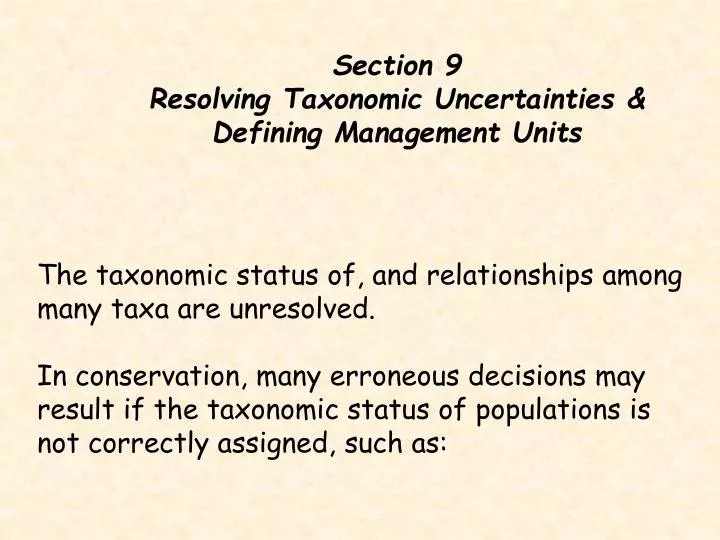
Section 9 Resolving Taxonomic Uncertainties & Defining Management Units. The taxonomic status of, and relationships among many taxa are unresolved. In conservation, many erroneous decisions may result if the taxonomic status of populations is not correctly assigned, such as:.

E N D
Section 9 Resolving Taxonomic Uncertainties & Defining Management Units The taxonomic status of, and relationships among many taxa are unresolved. In conservation, many erroneous decisions may result if the taxonomic status of populations is not correctly assigned, such as:
Unrecognized endangered species may be allowed to become extinct. Incorrectly diagnosed species may be hybridized with other species, resulting in reduced reproductive fitness. Resources may be wasted on abundant species, or hybrid populations.
Populations that could be used to improve the fitness of inbred populations may be overlooked. Endangered species may be denied legal protection while populations of common species, or hybrids between species, may be granted protection.
Recent molecular studies among sea turtles compared the Kemp’s ridley turtle (Lepidochelys kempi) and the similar olive ridley turtle (L. olivacea) and supported recognition of Kemp’s ridley turtle as a valid species. Studies of the genetics of minke whales (Balaenoptera acutorostrata) have led investigators to advocate that the Northern and Southern Hemisphere populations be treated as two distinct species (Hoelzel and Dover, 1991).
Similar conclusions were reached based on molecular studies of sympatric populations of killer whales (Orcinus orca). This case is particularly interesting because it suggests that observed differences in behavior in sympartric populations, so called “resource polymorphisms”, may be genetically based (Hoelzel 1998).
Proper identification and determination of evolutionary relationships can prevent hybridization, and sometimes genetic extinction of “look-alike” species.
Case of the Extinct Dusky Sea Side Sparrow 1872, a melanistic form of seaside sparrow was discovered in Brevard co. FL and described as a distinct species: Ammodramus nigrescens. 1960s the population (now a subspecies) was in severe decline due to habitat alterations and the Dusky Seaside Sparrow was placed on the U.S. Endangered Species List.
Currently, about 9 subspecies recognized with more or less abutting ranges along the species coastal-marsh habitat from New England to south Texas. 1980, the few remaining birds (all males) were brought into captivity and mated to individuals from a Gulf Coast population.
The objective was to produce F1 hybrids and then backcross progeny (the latter carrying primarily dusky nuclear genes) for eventual reintroduction. The breeding program was not successful and thus discontinued. Avis and Nelson (1989) assayed mtDNA haplotypes from 40 seaside sparrows representing 7 named subspecies and the last available dusky male, which died in captivity in 1987.
Gulf Coast haplotypes Atlantic Coast haplotypes 7 5 8 3 1 6 11 2 9 4 10 Most common Atlantic haplotype and haplotype of Dusky seaside sparrow
Thus, the traditional taxonomy for seaside sparrows, from which conservation priorities were derived, probably had been a misleading guide to evolutionary relationships in this complex for two reasons: in failure to recognize the fundamental phylogenetic dichotomy between Atlantic & Gulf populations. 2. in taxonomic emphasis on distinctions within both coastal regions that appear evolutionarily minor compared to the between-region genetic differences.
Captive breeding of gazelles and dik-diks that were supposedly of the same species ha sometimes produced infertile offspring. Subsequent cytogenetic analyses revealed that the parents were of different species.
Dealing specifically with dik-diks, Benirschke & Kumamoto (1991) noted that not only were individuals of different species bred together in captivity, but also hybrids of Kirk’s (Madoqua kirkii) and Guenther’s (M. rhyncotragus) dik-diks were found in 300 collections. These authors concluded that a cytogenetic analysis should be mandatory prior to captive breeding populations are established to eliminate unnecessary hybridization and reduced fertility.
Resolving Taxonomic Uncertainties
Phylogenetic trees are used to resolve taxonomic uncertainties. A phylogenetic tree is composed of lines called branches that intersect and terminate at nodes. The nodes at the tips of the branches represent the taxa that exist today and that we can actually examine. The internal nodes represent ancestral taxa, whose properties we can only infer from the existing data.
Rooted tree whose branch tips represent 5 taxa (A - E) in a clade, with 4 internal nodes (R, X, Y, Z) representing ancestral taxa, including the root (R). The numbers on branches indicate the number of changes in a particular sequence that occurred along that branch. These numbers represent the branch lengths. A 2 1 Z B 1 2 C 3 1 1 Y D R 7 E
Even if exact values are not provided, the relative lengths of the branches may be drawn in proportion to the number of changes along that branch. This tree is additive because the distance between any two nodes equals the sum of the lengths of all branches between them. If multiple substitutions have occurred at any site, then additivity will not hold unless distances are corrected for multiple substitutions. A 2 1 Z B 1 2 C 3 1 1 Y D R 7 E
A tree is said to be rooted if there is a particular node -- the root -- from which a unique directional path leads to each extant taxon. In this tree, R is the root because it is the only internal node from which all other nodes can be reached by moving forward (toward the tips). The root is the common ancestor of all taxa in the analysis. A 2 1 Z B 1 2 C 3 1 1 Y D R 7 E
Unrooted tree, such as these, specify only the relationships among the taxa, and DO NOT define evolutionary pathways. For 4 taxa, there are only 3 possible unrooted trees. Once a root is identified, 5 different rooted trees can be created for EACH of these unrooted trees, each with a distinctive branching pattern reflecting a different evolutionary history. C A D B B A D C C A B D
The number of possible trees, both rooted and unrooted, increases dramatically as the number of taxa increases. Let s be the number of taxa, the number of possible unrooted trees is: (2s - 5)! / [2s-3(s-3)!] the number of possible rooted trees is: (2s - 3)! / [2s-3(s-3)!]
Taxa unrooted rooted trees trees 4 3 15 8 13,395 135,135 10 2,027,025 34,459,425 22 1 x 10²³almost a mole of trees 50 3 x 1074more trees than atoms in the universe
Unrooted trees tell us only about phylogenetic relationships; they tell us nothing about the directions of evolution -- the order of descent. Rooted trees tell us about the order of descent from the root toward the tips of the tree. While unrooted trees are always more “correct” in that they don’t imply knowledge that we do not have, they are considerably less informative.
Alignment of DNA sequences A pair of sequences can be aligned by writing one above the other in such a way as to maximize the number of residues that match by introducing gaps into one or the other sequence. Biologically, these gaps are assumed to represent insertions or deletions that occurred as the sequences diverged from a common ancestor.
If we could insert as many gaps as we chose, we could align any two random, unrelated sequences so that all residues either matched perfectly or were across from a gap in the other sequence. Such an alignment would be meaningless!!! It is necessary to somehow constrain the number of gaps so that the resulting alignment makes biological sense.
To do this, a scoring system is used so that matching residues get some sort of positive numerical score, and gaps get some sort of negative score, or gap penalty. An alignment program seeks an arrangement that maximizes the net score. For nucleic acid alignments, matching residues usually get a score of 1 and mismatches get a score of 0.
Gap penalties are typically set by the user and typically there is a penalty for creating a gap plus an extra penalty for the length of the gap. Aligning a pair of sequences is not a computationally difficult process, and a variety of programs exist to align sequence pairs. Multiple alignments are considerably more complex, and only a few programs do a really good job. CLUSTALX is one of the best tools for creating multiple sequence alignments.
An alignment is not an absolute thing. It is a “best guess” according to some algorithm used by a computer program. One cannot simply have a program compute an alignment and, without further thought, use that alignment to create a phylogeny.
Distance Based Methods of Tree Construction In these methods, distances are expressed as the fraction of sites that differ between 2 sequences in a multiple alignment. It is fairly obvious that a pair of sequences differing at only 10% of their sites are more closely related than a pair differing at 30% of their sites. It also makes sense that the more time has passed since two sequences diverged from a common ancestor, the more the sequences will differ.
Although the latter assumption is reasonable, it is not always true. It might be untrue because one lineage evolved faster than the other. Even if two lineages evolved at the same rate, the assumption might be untrue because of multiple substitutions.
As two sequences diverge from a common ancestor, each nucleotide substitution initially will increase the number of differences between the two lineages. As those differences accumulate, however, it becomes increasingly likely that a substitution will occur at the same site where an earlier substitution occurred.
While there are statistical corrections used to estimate corrected distances from the number of observed differences, differences almost always underestimate the actual amount of change along lineages. The two most popular distance methods, UPGMA and Neighbor-Joining, are both algorithmic methods -- i.e., they use a specific series of calculations to estimate a tree.
The calculations involve manipulations of a distance matrix that is derived from a multiple alignment. Starting with the multiple alignment, both programs calculate for each pair of taxa the distance, or the fraction of differences, between the two sequences and write that distance to a matrix.
UPGMA: UPGMA (Unweighted Pair-Group Method with Arithmetic Mean) is an example of a clustering method. We covered this procedure in chapter 13. UPGMA has built into it an assumption that the tree is additive and that it is ultrametric -- all taxa are equally distant from a root -- an assumption that is very unlikely. For that and other reasons, UPGMA is rarely used today.
Neighbor-Joining (NJ): NJ is similar to UPGMA in that it manipulates a distance matrix, reducing it in size at each step, then reconstructs the tree from that series of matrices. It differs from UPGMA in that it does not construct clusters but directly calculates distances to internal nodes.
From the original matrix, NJ first calculates for each taxon its net divergence from all other taxa as the sum of the individual distances from the taxon. It then uses the net divergence to calculate a corrected distance matrix. NJ then finds the pair of taxa with the lowest corrected distance and calculates the distance from each of those taxa to the node that joins them.
A new matrix is then created in which the new node is substituted for those two taxa. NJ does not assume that all taxa are equidistant from a root. NJ is, like parsimony, a minimum-change method, but it does not guarantee finding the tree with the smallest overall distance.
Indeed, there are cases in which many shorter trees than the NJ exist. Some authors think that the best use of an NJ tree is as a starting point for a model-based analysis such as Maximum-likelihood.
Parsimony: Parsimony is based on the assumption that the most likely tree is the one that requires the fewest number of changes to explain the data. The basic premise of parsimony is that taxa sharing a common characteristic do so because they inherited that characteristic from a common ancestor.
When conflict occur, they are explained by reversal, convergence, or parallelism and these explanations are gathered under the term homoplasy. Homoplasies are regarded as “extra” steps or hypotheses that are required to explain the data. Parsimony operates by selecting the tree or trees that minimize the number of evolutionary steps, including homoplasies, required to explain the data.
Parsimony or minimum change, is the criterion for choosing the best tree. For protein or nucleotide sequences, the data are aligned sequences. Each site in each alignment is a character, and each character can have a different state in different taxa. Not all characters are useful in constructing a parsimony tree.
Invariant characters, those that have the same state in all taxa, are obviously useless and are ignored by parsimony. Also ignored are characters in which a state occurs in only on taxon. An algorithm is used to determine the minimum number of steps necessary for any given tree to be consistent with the data. That number is the score for the tree, and the tree or trees with the lowest score are most parsimonious.
The algorithm is used to evaluate a possible tree at each informative site. Consider a set of 6 taxa, named 1 -- 6. At some site (character) in the alignment, the states of that character are: 1 = A 2 = C 3 = A 4 = G 5 = G 6 = C
There are 105 possible unrooted trees of 6 taxa. We will pick one unrooted tree, but all will be evaluated by the computer. If we root this tree at taxon 1, we get the following tree: C 2 A 3 G 4 A 1 G 5 C 6
6C 5G 3A 4G W X 2C Y Z 1A The algorithm starts at a tip and moves to the interior node that connects to another tip. If the two tips have the same state, they assign that state to the node; if they do not, they assign an “or” state.
6C 5G 3A 4G W X 2C Y Z 1A Thus, node W is assigned the state A or G, and node X the state G or C. Node Y connects nodes W and X. Because the states at nodes W and X both include G, node Y is assigned the state G. Node Z is assigned the state C or G as follows:
6C 5G 3A 4G G or C A or G 2C G C or G 1A Once the root has been reached, the algorithm proceeds back up from the root toward the tips. Because node Z does not include the state at the node that is ancestral to it (taxon 1), its assignment is arbitrary
6C 5G 6C 3A 5G 4G 3A 4G G G 2C G or C A or G 2C G G G 1A C or G 1A Assume that it is assigned state G. Node Y is already assigned, so the algorithm moves to node W. Node W is assigned G because that assignment does not require a change from the node that is ancestral to it. Similarly, node X is assigned state G.
Each branch along which the state changed, indicated by thick branches, is counted. This tree has 4 changes. The other possible rootings of the tree are considered in the same way, and if a different rooting of the tree produces fewer changes, that is the score for that site. 5G 3A 4G G G 2C G G 1A
The parsimony program evaluates the tree for each informative site, then adds up the changes to calculate the minimum number of changes for that particular tree. As it works its way through the various possible trees, the program keeps track of the tree (or trees) with the lowest scores.
Evolutionary Models: Sequences diverge from a common ancestor because mutations occur and some fraction of those mutations are fixed into the evolving population by selection and by chance, resulting in the substitution of one nucleotide for another at various sites. To reconstruct evolutionary trees, we must make some assumptions about the substitution process and state those assumptions in the form of a model.