Download
1 / 24
240 likes | 244 Views
Hands-On Session: Regression Analysis. What we have learned so far Use data viewer ‘afni’ interactively Model HRF with a shape-prefixed basis function Assume the brain responds with the same shape in any active regions regardless stimulus types

E N D
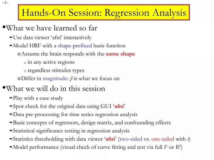
Hands-On Session: Regression Analysis • What we have learned so far • Use data viewer ‘afni’ interactively • Model HRF with a shape-prefixed basis function • Assume the brain responds with the same shape • in any active regions • regardless stimulus types • Differ in magnitude: β is what we focus on • What we will do in this session • Play with a case study • Spot check for the original data using GUI ‘afni’ • Data pre-processing for time series regression analysis • Basic concepts of regressors, design matrix, and confounding effects • Statistical significance testing in regression analysis • Statistics thresholding with data viewer ‘afni’ (two-sided vs. one-tailed with t) • Model performance (visual check of curve fitting and test via full F or R2)
Data Quality Check • To look at the data: typecd AFNI_data6/afni, then afni • Switch Underlay to dataset epi_r1 • Then AxialImage and Graph • FIMPick Ideal ; then click afni/epi_r1_ideal.1D ; then Set • Right-click in image, Jump to (ijk), then 26 72 4, then Set • Data clearly has activity in sync with reference • 20s blocks • Data also has a big spike at 89s • Head motion • Spike at t=0
Preparing Data for Analysis • Eight preparatory steps are common: • Outliers: 3dToutcount (or 3dTqual), 3dDespike • Temporal alignment or slice timing correction (sequential/interleaved): 3dTshift • Image/volume registration (aka realignment, head motion correction): 3dvolreg • Spatial normalization (standard space conversion): adwarp, @auto_tlrc, anlign_epi_anat.py • Blurring/smoothing: 3dmerge, 3dBlurToFWHM, 3dBlurInMask • Masking: 3dAutomask • Global mean scaling: 3dROIstats (or 3dmaskave) and 3dcalc • Temporal mean scaling: 3dTstat and 3dcalc • Not all steps are necessary or desirable in any given case
Data Analysis Script • 3dvolreg(3D image registration) will be covered in detail in a later presentation • filename to get estimated motion parameters • 3dDeconvolve = regression code • In file epi_r1_regress: 3dvolreg -base 3 \ -verb \ -prefix epi_r1_reg \ -1Dfile epi_r1_mot.1D \ epi_r1+orig 3dDeconvolve \ -input epi_r1_reg+orig \ -nfirst 2 \ -num_stimts 1 \ -stim_times 1 epi_r1_times.1D \ 'BLOCK(20)' \ -stim_label 1 AllStim \ -tout \ -bucket epi_r1_func \ -fitts epi_r1_fitts \ -xjpeg epi_r1_Xmat.jpg \ -x1D epi_r1_Xmat.x1D • Name of input dataset (from 3dvolreg) • Index of first sub-brick to process [skipping #0-1] • Number of input model time series • Name of input stimulus class timing file (’s) • and type of HRF model to fit • Name for results in AFNI menus • Indicates to output t-statistic for weights • Name of output “bucket” dataset (statistics) • Name of output model fit dataset • Name of image file to store X[AKA R] matrix • Name of text file in which to store X matrix • Type tcsh epi_r1_regress; then wait for programs to run
} MatrixQuality Assurance • 3dvolreg output • ++ 3dvolreg: AFNI version=AFNI_2009_12_31_1431 (Mar 18 2010) [64-bit] • ++ Reading input dataset ./epi_r1+orig.BRIK • ++ Edging: x=4 y=4 z=2 • ++ Creating mask for -maxdisp • + Automask has 66767 voxels • + 8103 voxels left in -maxdisp mask after erosion • ++ Initializing alignment base • ++ Starting final pass on 152 sub-bricks: 0..1..2..3.. ***..150..151.. • ++ CPU time for realignment=7.25 s [=0.0477 s/sub-brick] • ++ Min : roll=-0.006 pitch=-2.057 yaw=-0.019 dS=-0.090 dL=-0.028 dP=-0.116 • ++ Mean: roll=+0.039 pitch=-0.127 yaw=+0.022 dS=+0.059 dL=+0.030 dP=+0.042 • ++ Max : roll=+0.119 pitch=+0.013 yaw=+0.076 dS=+0.209 dL=+0.087 dP=+0.272 • ++ Max displacement in automask = 2.46 (mm) at sub-brick 42 • ++ Wrote dataset to disk in ./epi_r1_reg+orig.BRIK • 3dDeconvolve output • ++ 3dDeconvolve: AFNI version=AFNI_2009_12_31_1431 (Mar 18 2010) [64-bit] • ++ loading dataset epi_r1_reg+orig • *+ WARNING: Input polort=1; Longest run=304.0 s; Recommended minimum polort=3 • ++ -stim_times using TR=2 s for stimulus timing conversion • ++ Wrote matrix image to file epi_r1_Xmat.jpg • ++ Wrote matrix values to file epi_r1_Xmat.x1D • ++ ----- Signal+Baseline matrix condition [X] (150x3): 3.81681 ++ VERY GOOD ++ • ++ ----- Signal-only matrix condition [X] (150x1): 1 ++ VERY GOOD ++ • ++ ----- Baseline-only matrix condition [X] (150x2): 1.02336 ++ VERY GOOD ++ • ++ ----- polort-only matrix condition [X] (150x2): 1.02336 ++ VERY GOOD ++ • ++ +++++ Matrix inverse average error = 1.47717e-15 ++ VERY GOOD ++ • ++ Calculations starting; elapsed time=1.553 • ++ voxel loop:0123456789.0123456789.0123456789.0123456789.0123456789. • ++ Calculations finished; elapsed time=4.979 • ++ Wrote bucket dataset into ./epi_r1_func+orig.BRIK • + created 2 FDR curves in bucket header • ++ Wrote 3D+time dataset into ./epi_r1_fitts+orig.BRIK Screen Output of the epi_r1_decon script }Maximum movement estimate } Consider '-polort 3' }Output file indicators }Progress meter/pacifier }Output file indicators
Modeling Serial Correlation in the Residuals • Temporal correlation exists in the residuals of the time series regression model • Caused by physiological (respiratory, cardiac, and vasomotor) effects • First-order autocorrelation up to 0.4 in cortex • Within-subject variability (or statistical value) would get deflated (or inflated) if temporal correlation is not accounted for in the model • Should correct for the temporal correlation if bringing both effect size (β) and within- subject variability to group analysis • Doesn’t matter much if effect size is taken for group analysis • ARMA(1, 1) assumed in 3dREMLfit • Script automatically generated by 3dDeconvolve (may use –x1D_stop) • File epi_r1_func.REML_cmdunder AFNI_data6/afni • Run it by typing tcsh –x rall_func.REML_cmd 3dREMLfit -matrix epi_r1_Xmat.x1D -input epi_r1_reg+orig \ -tout -Rbuck epi_r1_func_REML -Rvar epi_r1_func_REMLvar \ -Rfitts epi_r1_fitts_REML -verb
Stimulus Timing: Input and Visualization X matrix columns epi_r1_times.txt=4 34 64 94 124 154 184 214 244 274 =times of start of each BLOCK(20) HRF copy • HRFtiming • Linear in t • All ones aiv epi_r1_Xmat.jpg 1dplot -sepscl epi_r1_Xmat.x1D
Look at the Activation Map • Run afni to view what we’ve got (N.B.: a weak test with only 1 run) • Switch Underlay to epi_r1_reg (background: input for 3dDeconvolve) • Switch Overlay to epi_r1_func (statistics: output from 3dDeconvolve) • Sagittal Image and Graph viewers (time series at a few voxels) • FIMIgnore2 to have graph viewer not plot 1st time point • FIMPick Ideal; pick epi_r1_ideal.1D (HRF: output from –x1D) • Define Overlay to set up functional coloring • OlayAllstim#0_Coef (sets coloring to be from : color spectrum) • ThrAllstim#0_Tstat (sets threshold to be t-statistic: slider bar) • See Overlay (otherwise won’t see the function!) – should be on automatically • Play with threshold slider to get a meaningful activation map (e.g., t(61)=3 is a decent threshold): what’s the difference between one- and two-sided? Which should be adopted? How to get one-side significance level on afni? • Again, use Jump to (i j k) to jump to index coordinates 26 72 4
Compare 3dDeconvolve and 3dREMLfit Group Analysis: will be carried out on or GLT coef (+t-value) from single-subject analysis
Visually check model performance • Graph viewer: OptTran 1DDataset #N to plot the model fit dataset output by 3dDeconvolve • Will open the control panel for the Dataset #N plugin • Click first Input line to be ‘on’; then choose Dataset epi_r1_reg+orig • Also choose Color dk-blue to get a pleasing plot • Click 2nd Input on; then choose Dataset epi_r1_fitts+orig • Also choose Color limegreen to get a pleasing plot • Then click on Set+Close(to close the plugin’s control panel) • This tool lets you visualize how the model performs
A Case Study • Speech Perception Task: Subjects were presented with audiovisual speech that was presented in a predominantly auditory or predominantly visual modality. • A digital video system was used to capture auditory and visual speech from a female speaker. • There were 2 types of stimulus conditions: (2) Visual-Reliable (1) Auditory-Reliable Example: Subjects can clearly hear the word “cat,” but the video of a woman mouthing the word is degraded. Example: Subjects can clearly see the video of a woman mouthing the word “cat,” but the audio of the word is degraded.
Experiment Design • 3 runs in a scanning session. • Each run consisted of 10 blocked trials: • 5 blocks contained Auditory-Reliable (Arel) stimuli, and • 5 blocks contained Visual-Reliable (Vrel) stimuli. • Each block contained 10 trials of Arel OR Vrel stimuli. • Each block lasted for 20s (1s for stimulus presentation, followed by a 1s inter-stimulus interval). • Each baseline block consisted of a 10s fixation point. 10 trials, 20sec 10 trials, 20sec 10 trials, 20sec 10 trials, 20sec 10 trials, 20sec etc… + + + + + 10sec 10sec 10sec 10sec 10sec
Data Collected • 2 anatomical datasets for each subject, collected from a 3T scanner • 124 axial slices • voxel dimensions = 0.938 x 0.938 x 1.2 mm • 3 time series (EPI) datasets for each subject • 33 axial slices x 152 volumes (TRs) per run • TR = 2s; voxel dimensions = 2.75 x 2.75 x 3.0 mm • Sample size, n = 10 (all right-handed subjects)
Regression Analysis • Run script by typing tcsh rall_regress (takes a few minutes) • 3dDeconvolve -input rall_vr+orig \ • -concat '1D: 0 150 300' \ • -num_stimts 8 \ • -stim_times 1 stim_AV1_vis.txt 'BLOCK(20,1)' -stim_label 1 Vrel \ • -stim_times 2 stim_AV2_aud.txt 'BLOCK(20,1)' -stim_label 2 Arel \ • -stim_file 3 motion.1D'[0]' -stim_base 3 -stim_label 3 roll \ • -stim_file 4 motion.1D'[1]' -stim_base 4 -stim_label 4 pitch \ • -stim_file 5 motion.1D'[2]' -stim_base 5 -stim_label 5 yaw \ • -stim_file 6 motion.1D'[3]' -stim_base 6 -stim_label 6 dS \ • -stim_file 7 motion.1D'[4]' -stim_base 7 -stim_label 7 dL \ • -stim_file 8 motion.1D'[5]' -stim_base 8 -stim_label 8 dP \ • -gltsym 'SYM: Vrel -Arel' -glt_label 1 V-A \ • -tout -x1D rall_X.xmat.1D -xjpeg rall_X.jpg \ • -fitts rall_fitts -bucket rall_func \ • -jobs 2 • 2 audiovisual stimulus classes were given using -stim_times • Important to include motion parameters as regressors? • May remove the confounding effects due to motion artifacts • 6 motion parameters as covariates via -stim_file + -stim_base • motion.1D generated from 3dvolreg with the -1Dfile option • Test the significance of head motion parameters • Switch from -stim_base to -stim_label roll … • Use -gltsym 'SYM: roll \ pitch \yaw \dS \dL \dP'
Modeling Serial Correlation in the Residuals • Temporal correlation exists in the residuals of the time series regression model • Within-subject variability (or statistical value) would get deflated (or inflated) if temporal correlation is not accounted for in the model • Better correct for the temporal correlation if bringing both effect size and within- subject variability to group analysis • ARMA(1, 1) assumed in 3dREMLfit • Script automatically generated by 3dDeconvolve (may use –x1D_stop) • File rall_func.REML_cmd under AFNI_data6/afni • Run it by typing tcsh –x rall_func.REML_cmd 3dREMLfit -matrix rall_X.xmat.1D -input rall_vr+orig \ -tout -Rbuck rall_func_REML -Rvar rall_func_REMLvar \ -Rfitts rall_fitts_REML -verb
} } Regressor Matrix for This Script (via -xjpeg) Head Motion Baseline Audiovisual stimuli } • 6 drift effect regressors • linear baseline • 3 runs times 2 params/run • 2 regressors of interest • 33 design • 6 head motion regressors • 3 rotations and 3 shifts aiv rall_xmat.jpg
Showing All Regressors (via -x1D) All regressors: 1dplot -sepscl rall_X.mat.1D
Showing Regressors of Interest Regressors of Interest: 1dplot rall_X.mat.1D’[6..7]’
Options in 3dDeconvolve - 1 -concat '1D: 0 150 300' • “File” that indicates where distinct imaging runs start inside the input file • Numbers are the time (TR) indexes inside the dataset file for start of runs • In this case, a text format .1D file put directly on the command line • Could also be a filename, if you want to store that data externally -num_stimts 8 • 2 audiovisual stimuli (+6 motion), thus 2 -stim_times below • Times given in the -stim_times files are local to the start of each run -stim_times 1 stim_AV1_vis.txt 'BLOCK(20,1)' -stim_label 1 Vrel • Content of stim_AV1_vis.txt 60 90 120 180 240 120 150 180 210 270 0 60 120 150 240 • Each of 3 lines specifies start time in seconds for stimuli within the run
Options in 3dDeconvolve - 2 -gltsym 'SYM: Vrel -Arel' -glt_label 1 V-A • GLTs:General Linear Tests • 3dDeconvolve provides test statistics for each regressor separately, but if you want to test combinations or contrasts of the weights in each voxel, you need the -gltsym option • Example above tests the difference between the weights for the Virual-reliable and the Audio-reliable responses • SYM: means symbolic input is on command line • Otherwise inputs will be read from a file • Symbolic names for each regressor taken from -stim_label options • Stimulus label can be preceded by + or - to indicate sign to use in combination of weights • Leave space after each label! • Goal is to test a linear combination of the weights • Null hypothesis Vrel =Arel • e.g., does Vrel get different response from Arel? • What do 'SYM: 0.5*Vrel +0.5*Arel’ and 'SYM: Vrel \ Arel’test?
Options in 3dDeconvolve - 4 -fout -tout = output both F- and t-statistics for each stimulus class (-fout) and stimulus coefficient (-tout)— but not for the baseline coefficients (use –bout for baseline) • The full model statistic is an F-statistic that shows how well all the regressors of interest explain the variability in the voxel time series data • Compared to how well just the baseline model time series fit the data times (in this example, have 24 baseline regressor columns in the matrix — 6 for the linear drift, plus 6 for motion regressors) • F = [SSE(r)–SSE(f)]df(n) [SSE(f)df(d)] • The individual stimulus classes also will get individual F- (if –fout added) and/or t-statistics indicating the significance of their individual incremental contributions to the data time series fit • If DF=1 (e.g., F for a single regressor), t is equivalent to F: t(n) = F2(1, n)
Results of rall_regress Script • Images showing results from third GLT contrast: VrelvsArel • Menu showing labels from 3dDeconvolve • Play with these results yourself!
Compare 3dDeconvolve and 3dREMLfit Group Analysis: will be carried out on or GLT coef (+t-value) from single-subject analysis