Download
1 / 12
120 likes | 120 Views
Learn how to graph polynomial functions by factoring them into linear factors and plotting the intercepts and turning points.

E N D
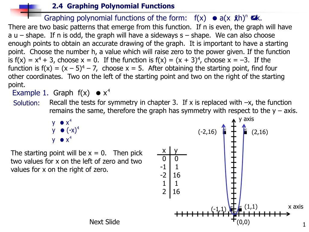
There are two basic patterns that emerge from this function. If n is even, the graph will have a u – shape. If n is odd, the graph will have a sideways s – shape. We can also choose enough points to obtain an accurate drawing of the graph. It is important to have a starting point. Choose the number h, a value which will raise zero to the power given. If the function is f(x) = x4 + 3, choose x = 0. If the function is f(x) = (x + 3)4, choose x = –3. If the function is f(x) = (x – 5)4 – 7, choose x = 5. After obtaining the starting point, find four other coordinates. Two on the left of the starting point and two on the right of the starting point. Recall the tests for symmetry in chapter 3. If x is replaced with –x, the function remains the same, therefore the graph has symmetry with respect to the y – axis. Solution: y axis (-2,16) (2,16) x y 0 0 -1 1 -2 16 1 1 2 16 (1,1) x axis (-1,1) Next Slide (0,0) The starting point will be x = 0. Then pick two values for x on the left of zero and two values for x on the right of zero.
y axis x y 3 0 2 1 1 16 4 1 5 16 (1,16) (5,16) x axis (2,1) (4,1) (3,0)
Solution: x y -1 0 -2 -1 -3 -8 0 1 1 8 y axis (1,8) (-1,0) x axis (0,1) (-2,-1) (-3,8) Next Slide Start with x = –1. Then pick two points to the left of –1 and two points to the right of –1.
x y 5 0 4 -1 3 -8 6 1 7 8 Graphing Polynomial Functions in Factored Form It is difficult to accurately graph most polynomial functions without using a calculator. A large number of points must be plotted to get a reasonably accurate graph. If a polynomial function P(x) can be factored into linear factors, its graph can be approximated by plotting only a few points. Using the factoring and graphing techniques available, a somewhat accurate graph can be achieved. For a complete discussion of graphing polynomial functions, tools of calculus will be needed which is beyond the scope of this course. Procedure for graphing polynomial functions in factored form: 1. Find all x intercepts (set all linear factors equal to zero). Plot the intercepts on the x-axis. 2. Find at least one point between the x intercepts and one point on left and right of the outer intercepts. 3. Draw in the graph describing the shape of the function.
y axis (4,15) x y -2 -15 0 3 2 -3 4 15 (0,3) x axis (1,0) (3,0) (-1,0) Note: (0,3) and (2,-3) are called turning points because the graph must turn to meet the next x intercept. A polynomial function of degree n has at most n – 1 turning points. This degree 3 polynomial has 2 turning points. Also, if the y value for the outside points is too large to plot, it is acceptable to only show the direction of the graph. (2,-3) Next Slide (-2,15) Set each linear factor equal to zero to obtain the x intercepts. Plot on axis. Next, find points between and on the outside of the intercepts. Plot those on the coordinate plane.
y axis (3,15) Intercepts at x=0, x=2, x=-2. (-1,3) x y 3 15 -3 -15 -1 3 1 -3 (2,0) (0,0) (-2,0) x axis (1,-3) (-3,-15)
f(x) (-1,4) x y -3 -48 -1 4 1/2 -5/16 2 -8 x (0,0) (-2,0) (1,0) Note: (-3,48) is not labeled. However the graph does follow in that direction. Also notice this degree 4 polynomial has 3 turning points. (2,-8) Next Slide Find and plot x intercepts on axis. These intercepts are called “zeros”. Find points between and on the outside of the intercepts. Plot those on the coordinate plane.
f(x) zeros at x=-2, x=0, x=1. x y -3 48 -1 - 4 1/2 5/16 2 8 x (-2,0) (0,0) (1,0) (-1,-4)
The previous examples were all polynomial functions in factored form. The next example will contain a polynomial function which is not in factored form. The polynomials will need to be factored first before the graphing procedure can be started. To factor, recall using the rational root theorem and the factor theorem from the previous section. f(x) (-1,0) x (2,0) x y 0 -2 1 -4 -2 -4 3 16 (-2,-4) (1,-4) Factor the polynomial using the rational root theorem and synthetic division. Now find the intercepts and graph the function.
f(x) Intercepts at x=-1, x=-3. (0,3) (-2,1) x y -4 -9 -2 1 0 3 x (-3,0) (-1,0) (-4,-9)
f(x) (-1,9) (3,9) x y 1 1 -1 9 3 9 (1,1) x (0,0) (2,0) Factor the polynomial using techniques of factoring from previous sections. Now find the intercepts and graph the function.
f(x) (2,16) Intercepts at x=0, x=1, x=-2. x y -3 -24 -1 4 1/2 -5/4 2 16 x (-2,0) (0,0) (1,0) (-3,-24) The End. B.R. 2-26-07