Download
1 / 55
560 likes | 567 Views
Partitioning and Divide-and-Conquer Strategies. Chapter 4. Introduction. In this chapter, we explore two of the most fundamental techniques in parallel programming: partitioning and divide-and-conquer.

E N D
Introduction • In this chapter, we explore two of the most fundamental techniques in parallel programming: partitioning and divide-and-conquer. • In partitioning, the problem is simply divided into separate parts and each part is computed separately. • Divide and conquer usually applies partitioning in a recursive manner by continually dividing the problem into smaller and smaller parts and combining the results.
1. Partitioning • 1.1 Partitioning Strategies • This is the basis for all parallel programming, in one form or another. • Embarrassingly parallel problems of the last chapter used partitioning. • Most partitioning formulations, however, require the results to be combined
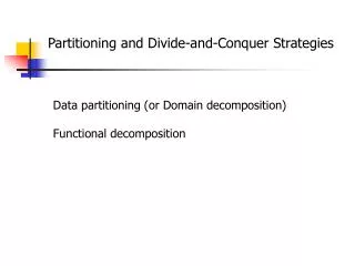
1. Partitioning • Partitioning can be applied to the program data • this is called data partitioning or domain decomposition • Partitioning can also be applied to the functions of the program • this is called functional decomposition • It is much less common to find concurrent functions in a program, but data partitioning is a main strategy for parallel programming.
1. Partitioning • Consider the problem of adding n numbers on m processors. • Each processor would add n/m numbers into a partial sum
1. Partitioning • How would you do this in a master-slave approach? • How would the slaves get the numbers? • One send per slave? • One broadcast?
1. Partitioning • Send-Receive Code: • Master: s = n/m; /* number of numbers for slaves*/ for (i = 0, x = 0; i < m; i++, x = x + s) send(&numbers[x], s, P i ); /* send s numbers to slave */ sum = 0; for (i = 0; i < m; i++) { /* wait for results from slaves */ recv(&part_sum, P_ANY ); sum = sum + part_sum; /* accumulate partial sums */ }
1. Partitioning • Slave recv(numbers, s, P_master ); /* receive s numbers from master */ part_sum = 0; for (i = 0; i < s; i++) /* add numbers */ part_sum = part_sum + numbers[i]; send(&part_sum, P_master ); /* send sum to master */
1. Partitioning • Broadcast Code • Master: s = n/m; /* number of numbers for slaves */ bcast(numbers, s, P slave_group );/* send all numbers to slaves */ sum = 0; for (i = 0; i < m; i++){ /* wait for results from slaves */ recv(&part_sum, P ANY ); sum = sum + part_sum; /* accumulate partial sums */ }
1. Partitioning • Broadcast Code • Slave bcast(numbers, s, P master ); /* receive all numbers from master*/ start = slave_number * s; /* slave number obtained earlier */ end = start + s; part_sum = 0; for (i = start; i < end; i++) /* add numbers */ part_sum = part_sum + numbers[i]; send(&part_sum, P master ); /* send sum to master */
1. Partitioning • Analysis • Phase 1 - Communication (numbers to slaves) • tcomm1 = m(tstartup + (n/m)tdata) • tcomm1 = tstartup + ntdata = O(n) • Phase 2 - Computation • tcomp1 = n/m -1 • Phase 3 - Communication • using individual sends: tcomm2 = m(tstartup + tdata) • using a gather - reduce: tcomm2 = tstartup + mtdata • Phase 4 - Computation • tcomp2 = m -1
1. Partitioning • Analysis (cont.) • Overall • tp = (m+1)tstartup +(n+m)tdata + m + n/m • tp = O(n+m) • We see that the parallel time complexity is worse than the sequential time complexity O(n)
1.2 Divide and Conquer • Characterized by dividing a problem into subproblems that are of the same form as the larger problem. • Further divisions into still smaller sub-problems are usually done by recursion • I know that one would never use recursion to add a list of numbers, but....the following discussion is applicable to any problem that is formulated by a recursive divide-and-conquer method.
1.2 Divide and Conquer • A sequential recursive definition for adding a list of numbers is int add(int *s) /* add list of numbers, s */ { if (number(s) =< 2) return (n1 + n2);/* see explanation */ else { Divide (s, s1, s2); /* divide s into two parts, s1 and s2 */ part_sum1 = add(s1); /*recursive calls to add sub lists */ part_sum2 = add(s2); return (part_sum1 + part_sum2); } }
1.2 Divide and Conquer • When each division creates two parts, we form a binary tree.
1.2 Divide and Conquer • Parallel Implementation • In a sequential implementation, only one node of the tree can be visited at a time. • A parallel solution offers the prospect of traversing several parts of the tree simultaneously. • This can be done inefficiently • have a processor for each node • therefore each processor is only active for one level in the tree computation. • Or efficiently • re-use processors
1.2 Divide and Conquer • Suppose we statically create eight processors (or processes) to add a list of numbers. • Process P 0 • /* division phase */ • divide(s1, s1, s2); /* divide s1 into two, s1 and s2 */ • send(s2, P 4 ); /* send one part to another process */ • divide(s1, s1, s2); • send(s2, P 2 ); • divide(s1, s1, s2); • send(s2, P 1 }; • part_sum = *s1; /* combining phase */ • recv(&part_sum1, P 1 ); • part_sum = part_sum + part_sum1; • recv(&part_sum1, P 2 ); • part_sum = part_sum + part_sum1; • recv(&part_sum1, P 4 ); • part_sum = part_sum + part_sum1;
1.2 Divide and Conquer • Process P 4 • recv(s1, P 0 ); /* division phase */ • divide(s1, s1, s2); • send(s2, P 6 ); • divide(s1, s1, s2); • send(s2, P 5 ); • part_sum = *s1; /* combining phase */ • recv(&part_sum1, P 5 ); • part_sum = part_sum + part_sum1; • recv(&part_sum1, P 6 ); • part_sum = part_sum + part_sum1; • send(&part_sum, P 0 ); • Other processes would require similar sequences
1.2 Divide and Conquer • Analysis • Communication • tcomm1 = n/2 tdata +n/4 tdata + n/8 tdata + ...+n/p tdata • tcomm1 = (n(p-1))/p tdata • Computation • tcomp = n/p + log p • Total • If p is constant we end up with O(n) • for large n and variable p, we end up with • tp = ((n(p-1))/p)tdata +tdata log p + n/p + log p
1.3 M-ary Divide and Conquer • Divide and conquer can also be applied where a task is divided into more than two parts at each stage. • Task broken into four parts. • The sequential recursive definition would be
1.3 M-ary Divide and Conquer int add(int *s) /* add list of numbers, s */ { if (number(s) =< 4) return(n1 + n2 + n3 + n4); else { Divide (s,s1,s2,s3,s4); /* divide s into s1,s2,s3,s4*/ part_sum1 = add(s1); /*recursive calls to add sublists */ part_sum2 = add(s2); part_sum3 = add(s3); part_sum4 = add(s4); return (part_sum1 + part_sum2 + part_sum3 + part_sum4); } }
1.3 M-ary Divide and Conquer • A tree in which each node has four children is called a quadtree.
1.3 M-ary Divide and Conquer • For example: a digitized image could be divided into four quadrants:
1.3 M-ary Divide and Conquer • An octree is a tree in which each node has eight children and has application for dividing a three-dimensional space recursively. • See Ben Lucchesi’s MS Thesis from 2002 for a parallel collision detection algorithm using octrees.
2. Divide-and-Conquer Examples • 2.1 Sorting Using Bucket Sort • Bucket sort is not based upon compare-exchange, but is naturally a partitioning method. • Bucket sort only works well if the numbers are uniformly distributed across a known interval (say 0 to a-1) • This interval will be divided into m regions, and a bucket is assigned to hold all the numbers within each region. • The numbers in each bucket will be sorted using a sequential sorting algorithm
2.1 Sorting Using Bucket Sort • Sequential Algorithm • place the numbers in their bucket • one time step per number -- O(n) • Sort the n/m numbers in each bucket • O(n/m log (n/m)) • If n = km, where k is a constant, we get O(n)
2.1 Sorting Using Bucket Sort • Note: • This is a much better than the lower bound for sequential compare and exchange sorting algorithms • However, it only applies when the numbers are well distributed.
2.1 Sorting Using Bucket Sort • Parallel Algorithm • Clearly, bucket sort can be parallelized by assigning one processor for each bucket.
2.1 Sorting Using Bucket Sort • But -- each processor had to examine each number, so a bunch of wasted effort took place. • We can improve this by having m small buckets at each processor and only looking at n/m numbers.
2.1 Sorting Using Bucket Sort • Analysis • Phase 1 - Computation and Communication • partition numbers into p regions, tcomp1 = n • send the data to the slaves, tcomm1 = tstartup + (tdata n) • If you can broadcast. • Phase 2 - Computation • separate n/p number into p small buckets, tcomp2 = n/p • Phase 3 - Communication • distribute small buckets, tcomm3 = (p-1)(tstartup+(n/p2)tdata) • Phase 4 - Computation • tcomp4 = (n/p)log(n/p) • Overall • tp = tstartup +tdatan + n/p + (p-1)(tstartup+(n/p2)tdata)+(n/p)log(n/p)
2.1 Sorting Using Bucket Sort • Phase 3 is basically an all-to-all personalized communication
2.1 Sorting Using Bucket Sort • You can do this in Mpi with MPI_Alltoall()
2.2 Numerical Integration • A general divide-and-conquer technique divides the region continually into parts and lets some optimization function decide when certain regions are sufficiently divided. • Let’s look now at our next example: • I = òab f (x) dx • To integrate (compute the area under the curve) we can divide the area into separate parts, each of which can be calculated by a separate process.
2.2 Numerical Integration • Each region could be calculated using an approximation given by rectangles:
2.2 Numerical Integration • A better approximation can be found by Aligning the rectangles:
2.2 Numerical Integration • Another improvement is to use trapezoids
2.2 Numerical Integration • Static Assignment -- SPMD pseudocode: • Process P i if (i == master) { /* read number of intervals required */ scanf(%d”,&n); printf(“Enter number of intervals ”); } bcast(&n, P group ); /* broadcast interval to all processes */ region = (b - a)/p; /* length of region for each process */ start = a + region * i; /* starting x coordinate for process */ end = start + region; /* ending x coordinate for process */ d = (b - a)/n; /* size of interval */ area = 0.0; for (x = start; x < end; x = x + d) area = area + f(x) + f(x+d); area = 0.5 * area * d; reduce_add(&integral, &area, P group ); /* form sum of areas */
2.2 Numerical Integration • Adaptive Quadrature • this method allows us to know how far to subdivide. • Stop when largest area is approximately = to sum of other 2.
2.2 Numerical Integration • Adaptive Quadrature (cont) • Some care might be needed in choosing when to terminate.
2.3 N-Body Problem • The objective is to find positions and movements of bodies in space (say planets) that are subject to gravitational forces from other bodies using Newtonian laws of physics. • The gravitational force between two bodies of masses maand mbis given by • F = (Gmamb)/(r2) • where G is the gravitational constant and r is the distance between the two bodies
2.3 N-Body Problem • Subject to forces, a body will accelerate according to Newton’s second law: • F = ma • where m is the mass of the body, • F is the force it experiences, • and a is the resultant acceleration.
2.3 N-Body Problem • Let the time interval be Dt. • Then, for a particular body of mass m, the force is given by • F= (m(vt+1-vt))/Dt • and a new velocity • vt+1 = vt + (FDt)/m • where vt+1 is the velocity of body at time t + 1 and vt is the velocity of body at time t.
2.3 N-Body Problem • If a body is moving at a velocity v over the time interval Dt, its position changes by • xt+1 -xt = vDt • where xtis its position at time t. • Once bodies move to new positions, the forces change and the computation has to be repeated.
2.3 N-Body Problem • Three-Dimensional Space • In a three-dimensional space having a coordinate system (x, y, z), the distance between the bodies at (xa, ya, za) and (xb, yb, zb) is given by • The forces are resolved in the three directions, using, for example,
2.3 N-Body Problem • Sequential Code for (t = 0; t < tmax; t++) /* for each time period */ for (i = 0; i < N; i++) { /* for each body */ F = Force_routine(i); /* compute force on ith body */ v[i]new = v[i] + F * dt / m;/* compute new velocity and x[i]new = x[i] + v[i]new * dt;/* new position (leap-frog) */ } for (i = 0; i < nmax; i++) { /* for each body */ x[i] = x[i]new ; /* update velocity and position*/ v[i] = v[i]new ; }
2.3 N-Body Problem • Parallel Code • The algorithm is an O(N2 ) algorithm (for one iteration) as each of the N bodies is influenced by each of the other N - 1 bodies. • Not feasible to use this direct algorithm for most interesting N-body problems where N is very large.
2.3 N-Body Problem • Time complexity can be reduced using the observation that a cluster of distant bodies can be approximated as a single distant body of the total mass of the cluster sited at the center of mass of the cluster:
2.3 N-Body Problem • Barnes-Hut Algorithm • Start with whole space in which one cube contains the bodies (or particles). • First, this cube is divided into eight subcubes. • If a subcube contains no particles, the subcube is • deleted from further consideration. • If a subcube contains more than one body, it is recursively divided until every subcube contains one body.