Download
1 / 67
1.09k likes | 1.97k Views
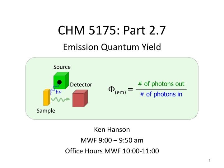
Emission Quantum Yield. CHM 5175: Part 2.7. Source. # of photons out. Detector. F ( em ) =. h n. # of photons in. Sample. Ken Hanson MWF 9:00 – 9:50 am Office Hours MWF 10:00-11:00. High Efficiency Emitters. Metal Ion Sensing. High Efficiency Emitters. High Efficiency Emitters.

E N D
Emission Quantum Yield CHM 5175: Part 2.7 Source # of photons out Detector F(em) = hn # of photons in Sample Ken Hanson MWF 9:00 – 9:50 am • Office Hours MWF 10:00-11:00
High Efficiency Emitters Metal Ion Sensing
High Efficiency Emitters Biological Labeling
High Efficiency Emitters OLED Samsung (10/9/13)
High Efficiency Emitters Expression Studies 4-(p-hydroxybenzylidene)- imidazolidin-5-one Green Fluorescent Protein
High Efficiency Emitters http://www.glofish.com/
Emission Quantum Yield Source Emission Quantum Yield (F) Detector hn # of photons emitted F= # of photons absorbed Sample Ground State (S0) Singlet Excited State (S1) hn hn
Excited State Decay Radiative Decay Excitation Non-emissive Decay Non-radiative Decay # of photons emitted F= # of photons absorbed
Excited State Decay Reaction Kinetics kr+knr kA S0 S1 S0 If it is assumed that all processes are first order with respect to number densities of S0 and S1 (nS0 and nS1in molecules per cm3) S1 Then the rate Equation: knr kr kA Energy kA= excitation rate kr= radiative rate knr= non-radiative rate S0
Excited State Decay Rate equation: Sample is illuminated with photons of constant intensity, a steady-state concentration of S1 is rapidly achieved. dnS1/dt = 0 S1 knr kr kA kA= excitation rate kr= radiative rate knr= non-radiative rate Energy Substitution for photon flux and the relationship between kA and kr then (math happens): S0 F = Emission Quantum Yield
Quantum Yield # of photons emitted = # of photons absorbed kr knr
Rate constants: kr = radiative kchem= photochemistry kdec = decomposition kET = energy transfer ket = electron transfer ktict = proton transfer ktict = twisted-intramolecular charge transfer kic = internal conversion kisc = intersystem crossing Non-radiative Rates kr FF= kr + knr kr FF= kr + kchem + kdec+ kET + ket + kpt + ktict + kic+ kisc …
Emission Quantum Yield Quantum Yield:
Emission Quantum Yield # of photons emitted F= = 0 to 1 # of photons absorbed
Fluorescence Quantum Yield kr FF= kr + kchem + kdec+ kET + ket + kpt + ktict + kic+ kisc … • 1) Internal conversion (kic) • -non radiative loss via collisions with solvent or via internal vibrations. • 2) Quenching • -interaction with solute molecules capable of quenching excited state • (kchem,kdec,kET,ket ) • 3) Intersystem Crossing Rate • 4) Temperature • - Increasing the temperature will increase of dynamic quenching • 5) Solvent • - viscosity, polarity, and hydrogen bonding characteristics of the solvent • -Increased viscosity reduces the rate of bimolecular collisions • 6) pH • - protonated or unprotonated form of the acid or base may be fluorescent • 7) Energy Gap Law
Intersystem Crossing S1 T2 T1 E Excitation Fluorescence Intersystem Crossing Phosphorescence Increase in strength of spin-orbit interaction S0 FPhosphorescence FFluorescence Atom Size ISC
Measuring Quantum Yield Source Detector hn Sample # of photons emitted = # of photons absorbed We don’t get to directly measure F, kr or knr! We do measure transmittance and emission intensity.
Measuring Quantum Yield “Absolute” Quantum Yield Relative Quantum Yield
Relative Quantum Yield # of photons emitted = # of photons absorbed Ifis proportional to the amount of the radiation from the excitation source that is absorbed and Ff. If = FfI0 (1-10-A) If = emission intensity Ff = quantum yield I0 = incident light intensity A = absorbance If ∝Ff If ∝ A
Relative Quantum Yield Ff∝ If If = FfI0 (1-10-A) If ∝ A Compare sample (S) fluorescence to reference (R). (1-10-AR) nS2 IS FS x = x IR FR (1-10-AS) nR2 Known Reported Measured F = quantum yield I = emission intensity A = absorbance n = refractive index
Relative Quantum Yield Absorption Emission Reference Emission (1-10-AR) nS2 IS FS AR x = x IR FR (1-10-AS) nR2 I AS Sample Emission Same instrument settings: excitation wavelength, slit widths, photomultiplier voltage…
Relative Quantum Yield (1-10-AR) nS2 IS FS x = x IR FR (1-10-AS) nR2 ? Excitation Snell’s Law: Sinqi ni = Detector no Sinqo Emission Sinqi2 nS2 = nR2 Sinqo2
Relative Quantum Yield Emission Detector Absorption Detector Source (1-10-AR) nS2 IS FS IF x = x P0 P IR FR (1-10-AS) nR2 Sample Scatter Reflectance
Relative Quantum Yield [Ru(bpy)3] 2Cl in H2O F = 0.042-0.063 [Ru(bpy)3] 2PF6 in MeCN F = 0.062-0.095
Relative Quantum Yield • Minimizing Error: • Sample/Reference with similar: • - Emission range • - Quantum yield • Same Solvent • Known Standard • Same Instrument Settings • - Excitation wavelength • - Slit widths • - PMT voltage (1-10-AR) nS2 IS FS x = x IR FR (1-10-AS) nR2
Absolute Quantum Yield # of photons emitted F= # of photons absorbed Source Detector Integrating Sphere
Absolute Quantum Yield Hamamatsu: C9920-02 (99% reflectance for wavelengths from 350 to 1650 nm and over 96% reflectance for wavelengths from 250 to 350 nm) Fig. 2. Schematic diagram of integrating sphere (IS) instrument for measuring absolute fluorescence quantum yields. MC1, MC2: monochromators, OF: optical fiber, SC: sample cell, B: buffle, BT-CCD: back-thinned CCD, PC: personal computer.
Instrumentation Hamamatsu: C9920-02G Absolute quantum yield measurement system
Absolute Quantum Yield Horiba QY Accessory
Data Acquisition • Set excitation l • Insert reference • - holder + solvent • Irradiate Reference • Detect output across • - excitation and emission • 5) Insert Sample • Holder + solvent + sample • 6) Repeat 3 and 4
Self Absorption/Filter Effect Anthracene
Self Absorption/Filter Effect Inner filter effect Fluorescence intensity (1-10-AR) nS2 IS FS x = x IR FR (1-10-AS) nR2 If = FfI0 (1-10-A) Concentration (M)
Quantum Yield and Lifetime Substitution for photon flux and the relationship between kA and kr then (math happens): Intrinsic or natural lifetime (tn): lifetime of the fluorophore in the absence of non-radiative processes 1 tn= kr Radiative Rate and Extinction Coefficient: Extinction Coefficient Radiative Rate kr = tn
n: refractive index of medium :position of theabsorption maxima in wavenumbers [cm-1] : absorption coefficient Strickler and Berg “Relationship between Absorption Intensity and Fluorescence Lifetime of Molecules” J. Chem. Phys. 1962, 37, 814. Strickler-Berg relation The relation of the radiative lifetime of the molecule and the absorption coefficient over the spectrum [ref. 5] Relationship between absorption intensity and fluorescence lifetime kr = tn
N1a : number of molecules in state 1a v 1a 2b : frequency of the transition Suppose a large number of molecules, immersed in a nonabsorbing medium with refractive index n, to be within a cavity in some material at temperature T, The radiation density within the medium is given by Planck’s blackbody radiation law, Relationship between Einstein A and B coefficients Blackbody Radiation -(1) By the definition of the Einstein transition probability coefficients, the rate of molecules going from lower state 1 to upper state 2 by absorption of radiation, -(2) Einstein transition probability coefficients The rate at which molecules undergo this downward transition is given by -(3) spontaneous emission probability induced emission probability At equilibrium the two rates must be equal, so by equating (2) and (3),
-(4) Relationship between Einstein A and B coefficients According to the Boltzmann distribution law, the numbers of molecules in the two states at equilibrium are related by Ratio of molecules in the ground and excited state -(5) Substitution of Eqs. (1) and (5) into (4) results in Einstein’s relation, -(6)
The radiation density in the light beam after it has passed a distance x cm through the sample, the molar extinction coefficient can be defined by Relationship B coefficient to Absorption coefficient Radiation Density Photons per distance C: concentration in moles per liter If a short distance dx is considered, the change in radiation density may be -(7) For simplicity, all the molecules will be assumed to be in the ground vibronic state, -(8) The number of molecules excited per second with energy hv is given by Excitations/second -(9)
Combining Eqs. (7), (8), and (9), it is found -(10) Probability of a single excitation transition Relationship B coefficient to Absorption coefficient the probability that a molecule in state 10 will absorb of energy hv and go to some excited state To obtain the probability of going to the state 2b, it must be realized that this can occur with a finite range of frequencies, and Eq. (10) must be integrated over this range. Then -(11) If the molecules are randomly oriented, the average probability of absorption for a large number of molecules, Eq (2) give a similar relation to (11) -(2) -(12) Probability for all excitation transitions The probability coefficient for all transitions to the electronic state 2 -(13)
The wavefunctions of vibronic states are functions of both the electronic coordinates x and the nuclear coordinates Q, -(14) Lifetime relationship for molecules If M(x) is the electric dipole operator for the electrons, the probability for induced Absorption or emission between two states is proportional to the square of the Matrix element of M(x) between two states -(15) Using (14), the integral in this expression can be Relating Excitation Probability to Relaxation Probability of atoms where Electronic transition moment integral for the transition Assuming the nuclei to be fixed in a position Q