Download
1 / 16
160 likes | 436 Views
FE analysis with plane stress and plane strain elements E. Tarallo, G. Mastinu POLITECNICO DI MILANO, Dipartimento di Meccanica. Summary. Subjects covered in this tutorial An introduction to plane stress and plane strain elements An introduction to convergence theory

E N D
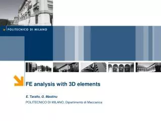
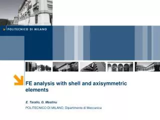
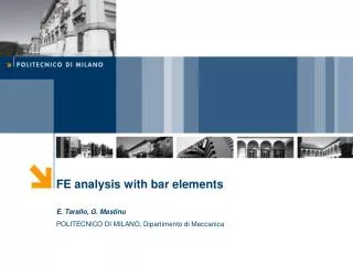
FE analysis with plane stress and plane strain elements E. Tarallo, G. Mastinu POLITECNICO DI MILANO, Dipartimento di Meccanica
Summary • Subjects covered in this tutorial • An introduction to plane stress and plane strain elements • An introduction to convergence theory • A guided example to evaluate a simple structure through the use of FEM • Comparison analytical vs numerical solutions • Other few exercises (to include in exercises-book)
Plane element – topic • Plane stress elements can be used when the thickness of a body is small relative to its lateral (in-plane) dimensions. The stresses are functions of planar coordinates alone, and the out-of-plane normal and shear stresses are equal to zero. Plane stress elements must be defined in the X–Y plane, and all loading and deformation are also restricted to this plane • Plane strain elements can be used when it can be assumed that the strains in a loaded body are functions of planar coordinates alone and the out-of-plane normal and shear strains are equal to zero. • DOF active: 1, 2 (translation of each node) • Output request: S11, S22, S33, S12
Convergence theory The Convergence Curve The formal method of establishing mesh convergence requires a curve of a critical result parameter (typically some kind of stress) in a specific location, to be plotted against some measure of mesh density. At least three convergence runs will be required to plot a curve which can then be used to indicate when convergence is achieved or, how far away the most refined mesh is from full convergence. Local Mesh Refinement All elements in the model should be split in all directions. It is not necessary to carry this out on the whole model: St Venant's Principle implies that local stresses in one region of a structure do not affect the stresses elsewhere. From a physical standpoint then, we should be able to test convergence of a model by refining the mesh only in the regions of interest, and retain the unrefined (and probably unconverged) mesh elsewhere. We should also have transition regions, from coarse to fine meshes, suitably distant from the region of interest
Exercise 1 Part: 3D shell planar Material: E=210 GPa, ν=0.3 Solution Type: Beam elements (no consider fillet) Plane elements (plane-stress or plane-strain?) 2.1 Tri linear 2.2 Tri quadratic 2.3 Quad linear 2.4 Quad quadratic Fine mesh (dimension 10mm) Coarse mesh (dimension 120mm) 3-Analytical solution B 1kN Thickness=10mm A For each configuration find: Max S22 in A Max displacement in B (magnitude & U2)
Exercise 2 Material: E=210 GPa, ν=0.3 Thickness=10mm Load: 1 kN (as ex1) Element: Quad quadratic Find Max MisesStress Fine mesh
Exercise 2 - modeling 1- Make 3 different Parts: 2- Insert them as 3 instances in Assembly 3- Use Translate Command (leave a gap between the faces)
Exercise 2 - interaction 4- Tie Connections 5- In the assembly fill the gap with translator command
Exercise 3 Part: 3D shell planar Material: E=210 GPa, ν=0.3 Load: σ0=1 Mpa Solution Type: plane elements Quad quadratic Goal: Find the stress filed around the hole and compare it with the analytical solution Find the number of elements that gives convergence Coarse and finer mesh, quadrilateral elements
Exercise 3 – analytical solution The analytical solution of the problem considering a circular hole in an infinite thin plate: Concentration coefficient Analyzing the trend of σθ on the contour of a hole with the radius a gives the maximum values in correspondence of π / 2 and 3π / 2.
Appendix – visualize different field output Displaying the results VISUALIZE, is the module that allows you to analyze the results of the analysis
Appendix – create a path Create path, defines a set of nodes from which you can extract the values of the magnitude of the desired output (stress, strain, temperature, etc.)
Appendix – create XY data and plot XY Data from path, plots the magnitudes of chosen parameters according to the previously selected nodes on the path Save the data of the plot: Using >Report>XY save the data in a report file Visualize directly the plot