Download
1 / 58
660 likes | 924 Views
Physics of the Atmosphere Physik der Atmosphäre. SS 2010 Ulrich Platt Institut f. Umweltphysik R. 424 Ulrich.Platt@iup.uni-heidelberg.de. Contents. Last Week.

E N D
Physics of the Atmosphere Physik der Atmosphäre SS 2010 Ulrich Platt Institut f. Umweltphysik R. 424 Ulrich.Platt@iup.uni-heidelberg.de
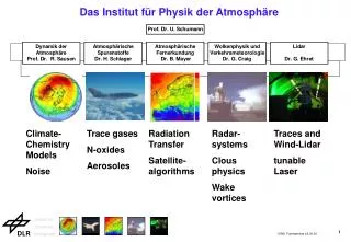
Last Week • Characteristice for measurement techniques for atmospheric trace gases: Sensitivity, Specific Detection, Spatial Coverage, Temporal Resolution, Stability of the Calibration, etc. • Diversity of measurement tasks: • Long Term Observations (note ‘operator dilemma’)(e.g. Stratospheric ozone trend, Change of Stratospheric chemistry (NDACC), Stratospheric (chlorine) source-gases, Tropospheric ozone trend (GAW), Greenhouse gase) • Regional Episodic Events(e.g. Pollution monitoring, Urban plume evolution, Continental plumes, Antarctic Ozone Hole, Polar boundary-layer ozone loss events) • Fast in-situ (Photo)chemistry (process studies)(e.g. Free radical (OH/HO2) photochemistry) • Measurement techniques: • Specialised (in-situ O3, NOX, etc.) • Universal: Mass-Spectroscopy • Optical spectroscopy • Gas-chromatography
invisible visible Rayleigh scatt. Mie scatt. Bio-Particles Viruses Bacteria Smoke Dust Storms Beach Sand Aitken Part. CCN Cloud Droplets Raindrops 0.001 0.01 0.1 1 10 100 1000 size (microns) Sizes of different Aerosol Particles An aerosol is a dispersion of solid and liquid particles suspended in gas
Physics of Aerosols, Part II • Optical properties • Measurement techniques
4. Optical Properties of the Aerosol Question: Why do we see aerosol particles, but not air molecules?(Example: cooling moist air produces a cloud or haze, what is different?)
1 10 0 Rayleigh regime 10 -1 10 Mie regime -2 10 Scattering eff. Qscatt=σscatt/πr2 -3 10 pol. parallel -4 10 pol. perpend. -5 10 -6 10 -7 10 0.01 0.1 1 10 Aerosol Optics Compare particle size and wavelength of light: α= 2pr/l : Size parameter α << 1 for molecules and fine particles: Rayleigh Scattering α ~>1 for coarse particles and clouds: Mie Scattering Scattering Coeff.:
Extinction of Radiation by Aerosol Homogeneous cloud of monodisperse aerosols with number concentration n and diameter Dp (Lambert-Beer) εext(λ): Extinction coefficient of the aerosol ensemble in m-1. σext(λ): Extinction cross section of individual aerosol particles in m2. Qext(λ): Q-Factor of individual aerosol particles as defined above. Similar relations are defined for scattering and absorption. With aerosol at number size distribution n(Dp), the extinction coefficient is or, in terms of the aerosol mass distribution:
Rayleigh Scattering Scattering cross section sR: according to Rayleigh theory: For molecules For small spheres: m: complex index of refraction
Epar Eperp Angular distribution fo the scattered Light:The Rayleigh Phase Function
Epar Mie Scattering • Scattering cross section sM: only applicable to spheres: Phase Function is complicated and strongly peaked in forward direction: (note log- scale)
Mie Phase Extinction Efficiency for Water Droplets Wavelength = 500nm, Radius varied Radius = 1 m, Wavelength varied Bohren & Huffman 1983
Mie Scattering Phase Functions Size Parameter: = 2r/ = Wavelength
From Mie and Rayleigh Theory to Atmospheric Optics Scattering / extinction coefficient = n·s (sometimescalled b) n: number of scatterers per unit volume s: scattering/extinction cross section (Rayleigh / Mie ) 1/: scattering mean free path definition of optical thickness τ (physical thickness in units of mean free path) Optical density Vertical optical density = „optical depth“
A0 Observer A(x) AE x L dx Visibility in the Atmosphere I When looking at a the black object (area A0) the scattered radiation intensity IR received by the observer (area AE) is given by:
Visibility in the Atmosphere II With the intensity IS: scattered within a volume element with area A(x) and thickness dx at distance x from the observer and ε: scattering coefficient. is a constant) Intensity received by the observer from volume Adx: Integration yields the total radiation flux received by the observer: For L the received intensity IR must be equal to the background intensity I0, so we obtain: The relative difference between the radiation intensity received from the black object IR compared to the flux I0 from its surrounding, the contrast C is given by: Visibility range Lv C=0.01 – 0.02:
Mass Scattering Efficiencies Scattering Efficiency too low Particle Area too low Seinfeld&Pandis
Aerosol Optical Depth (at 865 nm from Polder on ADEOS)IPCC (a) Aerosol optical depth and (b) Ångström exponent (AE) from POLDER satellite data for May 1997 (Deuzé et al., 1999). The largest optical depths over the Atlantic Ocean are from north African dust. The AE expresses the wavelength dependence of scattered light between 670 and 865 nm. The African dust plume has a small AE due to the importance of coarse mode aerosols whereas the larger AE‘s around the continents indicate accumulation mode aerosols there.
Annual Mean Direct Radiative Forcing by Anthropogenic SO4 Aerosol W/m2 Calculations by Roberts 1996
Solar and Infrared Forcing by Mineral Dust as a Function of Latitude Net heating! IR-Forcing Solar Forcing Tegen et al. Nature 1996
Mean Free Path in Gases The mean free path is defined as the average distance of molecules travelled between successive collisions where nz is the average collision frequency, n the number concentration of molecules, and dm the collision diameter of the molecules. For air dm = 0.37 nm = 3.7 Å. Size and spacing of air molecules at standard conditions Properties of air molecules at standard conditions
The Stopping Relaxation Time (Bremsrelaxationszeit) We assume that the aerosol particle is moving with velocity v relative to the carrier gas (being at rest).Since the braking force FSt v the particle will experience the „braking acceleration“: The constant KBr must have the dimension of an inverse time, thus: with = stopping time The above Differential equation has the simple solution: With v0 = initial velocity of the particle
Mobility of Aerosol Particles 3. Stopping Distance : The total distance covered by a by a particle with the initial velocity v0 given by: 4. Mobility B of a Particle: with see above m = mass of particlewe obtain: Conversely: v = -B F B is (like ) independent of the velocity (provided there is Stokes friction) and a characteristic quantity of the aerosol particle.
Overview of Aerosol measurement techniques • Number concentration (CPC) • Optical particle counters 2) Size Distribution Measurements • Impactors (cascade, ELPI, cyclone, CVI) • Differential mobility analyser (DMA, DMPS, SMPS) • Aerodynamic particle sizer (APS) 3)Aerosol Mass and chemical composition • Filter sampling techniques • Mass spectrometric techniques Sampling artefacts (isokinetic sampling, sampling losses)
Optical Particle Counters (OPC) PCS2000 optical particle counter Welas system from Palas GmbH, Karlsruhe: Principle: Particles fly through a very small, illuminated volume VM. VM is chosen that the probability of more than one particle being in the volume is very small.
Aerodynamic particle sizer (APS) Principle: Like OPC. Two laser beams allow to measure acceleration and thus B of the particle Size from: B-1F r
Condensation particle counter (CPC) The CPC (or Condensation Nucleus Counter, CNC) counts particles with a diameter of a few nanometres up to about one micrometer. The diameter of the particles is increased by condensational growth of supersaturated alcohol vapour before detection. The resulting uncontrolled increase in mass and therefore diameter makes it impossible to size classify the particle directly. Principle: Like OPC but grow small (optically invisible) particles by condensation of vapour.
Size Distribution - Measurement Techniques I • Impactors • Cascade Impactors
Size Distribution - Measurement Techniques II • Optical Particle Counter (OPC) • Microscopy (SEM, STM) • Mobility Analyser (e.g. DMA) • Condensation Particle Counter
Electrical Mobility Analyser In an electric field E, a particle carrying n elementary charges experiences a force F=neE that is balanced by the drag force: The terminal electrostatic velocity is given by The DMA system selects particles with electrical mobility where Ft and Fae are the total and aerosol flow rates, r1 and r2 are the inner and outer electrode radii, l is the length of the DMA and U is the voltage between the two electrodes.
Particle filters CNC or electrometer detector Differential MobilityAnalyzer (DMA) TSI
Comparison of measured aerosol behaviour in a cylindrical vessel with results from an aerosol process model
Electrical low pressure impactor (ELPI) The particle collection into each impactor stage is dependent on the aerodynamic size of the particles. Measured current signals are converted to (aerodynamic) size distribution using particle size dependent relations describing the properties of the charger and the impactor stages.
Aerodynamic particle sizer (APS) Number size distribution Mass size distribution (ρ = 2.6 g/cm3)
Filter sampling techniques Sampling on fiber filters by: Interception Impaction Diffusion
Particle Mass Spectrometer Aerodyne
Isokinetic sampling Sampling artefacts like can be avoided by isokinetic sampling configuration: The sampling tube is aligned to the streamlines and the is no change in velocity
Sampling efficiency Sedimentational losses in linear tubes