Download
1 / 32
350 likes | 1.21k Views
Lecture 4 – Classification of Flows Applied Computational Fluid Dynamics. Instructor: André Bakker. © Andr é Bakker (2002-2005) © Fluent Inc. (2002). Classification: fluid flow vs. granular flow. Fluid and solid particles: fluid flow vs. granular flow.

E N D
Lecture 4 – Classification of FlowsApplied Computational Fluid Dynamics Instructor: André Bakker © AndréBakker (2002-2005) © Fluent Inc. (2002)
Classification: fluid flow vs. granular flow • Fluid and solid particles: fluid flow vs. granular flow. • A fluid consists of a large number of individual molecules. These could in principle be modeled as interacting solid particles. • The interaction between adjacent salt grains and adjacent fluid parcels is quite different, however.
Reynolds number • The Reynolds number Re is defined as: Re = r V L / m. • Here L is a characteristic length, and V is the velocity. • It is a measure of the ratio between inertial forces and viscous forces. • If Re >> 1 the flow is dominated by inertia. • If Re << 1 the flow is dominated by viscous effects.
Effect of Reynolds number Re = 0.05 Re = 10 Re = 200 Re = 3000
Newton’s second law • For a solid mass: F = m.a • For a continuum: • Expressed in terms of velocity field u(x,y,z,t). In this form the momentum equation is also called Cauchy’s law of motion. • For an incompressible Newtonian fluid, this becomes: • Here p is the pressure and m is the dynamic viscosity. In this form, the momentum balance is also called the Navier-Stokes equation. Force per volume (body force) Mass per volume (density) Force per area (stress tensor) acceleration
Scaling the Navier-Stokes equation • For unsteady, low viscosity flows it is customary to make the pressure dimensionless with rV2. This results in:
Euler equation • In the limit of Re the stress term vanishes: • In dimensional form, with m = 0, we get the Euler equations: • The flow is then inviscid.
Scaling the Navier-Stokes equation - viscous • For steady state, viscous flows it is customary to make the pressure dimensionless with mV/L. This results in:
Navier-Stokes and Bernoulli • When: • The flow is steady: • The flow is irrotational: the vorticity • The flow is inviscid: μ = 0 • And using: • We can rewrite the Navier-Stokes equation: as the Bernoulli equation:
Basic quantities • The Navier-Stokes equations for incompressible flow involve four basic quantities: • Local (unsteady) acceleration. • Convective acceleration. • Pressure gradients. • Viscous forces. • The ease with which solutions can be obtained and the complexity of the resulting flows often depend on which quantities are important for a given flow. (steady laminar flow) (impulsively started) (boundary layer) (inviscid) (inviscid, impulsively started) (steady viscous flow) (unsteady flow)
Steady laminar flow • Steady viscous laminar flow in a horizontal pipe involves a balance between the pressure forces along the pipe and viscous forces. • The local acceleration is zero because the flow is steady. • The convective acceleration is zero because the velocity profiles are identical at any section along the pipe.
Flow past an impulsively started flat plate of infinite length involves a balance between the local (unsteady) acceleration effects and viscous forces. Here, the development of the velocity profile is shown. The pressure is constant throughout the flow. The convective acceleration is zero because the velocity does not change in the direction of the flow, although it does change with time. Flow past an impulsively started flat plate
Boundary layer flow along a finite flat plate involves a balance between viscous forces in the region near the plate and convective acceleration effects. The boundary layer thickness grows in the downstream direction. The local acceleration is zero because the flow is steady. Boundary layer flow along a flat plate
Inviscid flow past an airfoil involves a balance between pressure gradients and convective acceleration. Since the flow is steady, the local (unsteady) acceleration is zero. Since the fluid is inviscid (m=0) there are no viscous forces. Inviscid flow past an airfoil
Impulsively started flow of an inviscid fluid in a pipe involves a balance between local (unsteady) acceleration effects and pressure differences. The absence of viscous forces allows the fluid to slip along the pipe wall, producing a uniform velocity profile. The convective acceleration is zero because the velocity does not vary in the direction of the flow. The local (unsteady) acceleration is not zero since the fluid velocity at any point is a function of time. Impulsively started flow of an inviscid fluid
Steady viscous flow past a circular cylinder involves a balance among convective acceleration, pressure gradients, and viscous forces. For the parameters of this flow (density, viscosity, size, and speed), the steady boundary conditions (i.e. the cylinder is stationary) give steady flow throughout. For other values of these parameters the flow may be unsteady. Steady viscous flow past a cylinder
Unsteady flow past an airfoil at a large angle of attack (stalled) is governed by a balance among local acceleration, convective acceleration, pressure gradients and viscous forces. A wide variety of fluid mechanics phenomena often occurs in situations such as these where all of the factors in the Navier-Stokes equations are relevant. Unsteady flow past an airfoil
Flow classifications • Laminar vs. turbulent flow. • Laminar flow: fluid particles move in smooth, layered fashion (no substantial mixing of fluid occurs). • Turbulent flow: fluid particles move in a chaotic, “tangled” fashion (significant mixing of fluid occurs). • Steady vs. unsteady flow. • Steady flow: flow properties at any given point in space are constant in time, e.g. p = p(x,y,z). • Unsteady flow: flow properties at any given point in space change with time, e.g. p = p(x,y,z,t).
Newtonian fluids: water, air. Pseudoplastic fluids: paint, printing ink. Dilatant fluids: dense slurries, wet cement. Bingham fluids: toothpaste, clay. Casson fluids: blood, yogurt. Visco-elastic fluids: polymers (not shown in graph because viscosity is not isotropic). Newtonian (high μ) Bingham-plastic Casson fluid 0 Pseudo-plastic (shear-thinning) c Newtonian (low μ) Dilatant (shear-thickening) Strain rate (1/s) Newtonian vs. non-Newtonian (Pa)
Flow classifications • Incompressible vs. compressible flow. • Incompressible flow: volume of a given fluid particle does not change. • Implies that density is constant everywhere. • Essentially valid for all liquid flows. • Compressible flow: volume of a given fluid particle can change with position. • Implies that density will vary throughout the flow field. • Compressible flows are further classified according to the value of the Mach number (M), where. • M < 1 - Subsonic. • M > 1 - Supersonic.
Flow classifications • Single phase vs. multiphase flow. • Single phase flow: fluid flows without phase change (either liquid or gas). • Multiphase flow: multiple phases are present in the flow field (e.g. liquid-gas, liquid-solid, gas-solid). • Homogeneous vs. heterogeneous flow. • Homogeneous flow: only one fluid material exists in the flow field. • Heterogeneous flow: multiple fluid/solid materials are present in the flow field (multi-species flows).
Flow configurations - external flow • Fluid flows over an object in an unconfined domain. • Viscous effects are important only in the vicinity of the object. • Away from the object, the flow is essentially inviscid. • Examples: flows over aircraft, projectiles, ground vehicles.
Flow configurations - internal flow • Fluid flow is confined by walls, partitions, and other boundaries. • Viscous effects extend across the entire domain. • Examples: flows in pipes, ducts, diffusers, enclosures, nozzles. car interior airflow temperature profile
Classification of partial differential equations • A general partial differential equation in coordinates x and y: • Characterization depends on the roots of the higher order (here second order) terms: • (b2-4ac) > 0 then the equation is called hyperbolic. • (b2-4ac) = 0 then the equation is called parabolic. • (b2-4ac) < 0 then the equation is called elliptic. • Note: if a, b, and c themselves depend on x and y, the equations may be of different type, depending on the location in x-y space. In that case the equations are of mixed type.
Origin of the terms • The origin of the terms “elliptic,” “parabolic,” or “hyperbolic” used to label these equations is simply a direct analogy with the case for conic sections. • The general equation for a conic section from analytic geometry is: where if. • (b2-4ac) > 0 the conic is a hyperbola. • (b2-4ac) = 0 the conic is a parabola. • (b2-4ac) < 0 the conic is an ellipse.
Elliptic problems • Elliptic equations are characteristic of equilibrium problems, this includes many (but not all) steady state flows. • Examples are potential flow, the steady state temperature distribution in a rod of solid material, and equilibrium stress distributions in solid objects under applied loads. • For potential flows the velocity is expressed in terms of a velocity potential: u=f. Because the flow is incompressible, .u=0, which results in 2f=0. This is also known as Laplace’s equation: • The solution depends solely on the boundary conditions. This is also known as a boundary value problem. • A disturbance in the interior of the solution affects the solution everywhere else. The disturbance signals travel in all directions. • As a result, solutions are always smooth, even when boundary conditions are discontinuous. This makes numerical solution easier!
t=0 T=T0 t T=T0 x=L x=0 Parabolic problems • Parabolic equations describe marching problems. This includes time dependent problems which involve significant amounts of dissipation. Examples are unsteady viscous flows and unsteady heat conduction. Steady viscous boundary layer flow is also parabolic (march along streamline, not in time). • An example is the transient temperature distribution in a cooling down rod: • The temperature depends on both the initial and boundary conditions. This is also called an initial-boundary-value problem. • Disturbances can only affect solutions at a later time. • Dissipation ensures that the solution is always smooth.
Hyperbolic problems • Hyperbolic equations are typical of marching problems with negligible dissipation. • An example is the wave equation: • This describes the transverse displacement of a string during small amplitude vibrations. If y is the displacement, x the coordinate along the string, and a the initial amplitude, the solution is: • Note that the amplitude is independent of time, i.e. there is no dissipation. • Hyperbolic problems can have discontinuous solutions. • Disturbances may affect only a limited region in space. This is called the zone of influence. Disturbances propagate at the wave speed c. • Local solutions may only depend on initial conditions in the domain of dependence. • Examples of flows governed by hyperbolic equations are shockwaves in transonic and supersonic flows.
Classification of fluid flow equations • For inviscid flows at M<1, pressure disturbances travel faster than the flow speed. If M>1, pressure disturbances can not travel upstream. Limited zone of influence is a characteristic of hyperbolic problems. • In thin shear layer flows, velocity derivatives in flow direction are much smaller than those in the cross flow direction. Equations then effectively contain only one (second order) term and become parabolic. Also the case for other strongly directional flows such as fully developed duct flow and jets.
Blunt-nosed body designs are used for supersonic and hypersonic speeds (e.g. Apollo capsules and spaceshuttle) because they are less susceptible to aerodynamic heating than sharp nosed bodies. There is a strong, curved bow shock wave, detached from the nose by the shock detachment distance δ. Calculating this flow field was a major challenge during the 1950s and 1960s because of the difficulties involved in solving for a flow field that is elliptic in one region and hyperbolic in others. Today’s CFD solvers can routinely handle such problems, provided that the flow is calculated as being transient. Bow Shock M > 1 Hyperbolic region M < 1 M > 1 Blunt-nosed body δ Elliptic region Sonic Line Example: the blunt-nosed body
Initial and boundary conditions • Initial conditions for unsteady flows: • Everywhere in the solution region r, u and T must be given at time t=0. • Typical boundary conditions for unsteady and steady flows: • On solid walls: • u = uwall (no-slip condition). • T=Twall (fixed temperature) or kT/n=-qwall (fixed heat flux). • On fluid boundaries. • For most flows, inlet: r, u, and T must be known as a function of position. For external flows (flows around objects) and inviscid subsonic flows, inlet boundary conditions may be different. • For most flows, outlet: -p+mun/n=Fn and mut/n=Fn (stress continuity). F is the given surface stress. For fully developed flow Fn=-p (un/n =0) and Ft=0. For inviscid supersonic flows, outlet conditions may be different. • A more detailed discussion of boundary conditions will be given later on.
Summary • Fluid flows can be classified in a variety of ways: • Internal vs. external. • Laminar vs. turbulent. • Compressible vs. incompressible. • Steady vs. unsteady. • Supersonic vs. transonic vs. subsonic. • Single-phase vs. multiphase. • Elliptic vs. parabolic vs. hyperbolic.