Download
1 / 42
420 likes | 523 Views
AY202a Galaxies & Dynamics Lecture 13: LF Con’t, Galaxy Centers. Stepwise Maximum Likelihood. 1988 Efstathiou, Ellis & Peterson introduced SWML to get the form of the LF w/o “any” assumption about its shape. Parameterize LF as N p steps φ (L) = φ k

E N D
AY202a Galaxies & DynamicsLecture 13: LF Con’t,Galaxy Centers
Stepwise Maximum Likelihood 1988 Efstathiou, Ellis & Peterson introduced SWML to get the form of the LF w/o “any” assumption about its shape. Parameterize LF as Np steps φ(L) = φk Lk – ΔL/2 < L < Lk + ΔL/2
ln L = ∑ W((Li-Lk)ln k - ∑ ln {∑ j L H[Lj-Lmin(zi)]} + C Where N = number of galaxies in sample W(x) = 1 for - L/2 < L < +L/2 = 0 otherwise H(x) = 0 for x - L/2 = x/ L + 1/2 for -L/2 < L < +L/2 = 1 for x > L/2 Normalization via several techniques.
CfA1 Marzke et al. (1994)
LF in Clusters Smith, Driver & Phillips 1997 α = -1.8 at the faint end….
LCRS 1996 Lin et al. 1996
Current State of LF Studies 2dF blue photo ~250,000 gals, AAT Fibers SDSS red++ CCD, ~650,000 gals SDSS Fibers 2MASS JHK HgCdTe, 40,000 gals one of + 6dF fibers Stellar Masses from population synthesis
SDSS Mass Function vs Density Blanton & Moustakas (2009)
SDSS LF in Other Properties From Blanton Galex HI
Another Bias ---- we are in a special place There is excess clustering of galaxies around galaxies described often in terms of the correlation function ξ(r) = (r/r0)γ So the excess # of galaxies can be described by NE/N = 4 ∫ r2-γ r 0γ dr with this description we can correct the effective volume around US Vc = cV0 where c = 1 + 4 r0γ /(3-γ) 2r0 3-γ/V0 V0 = 4/3 r3
2MRS LF E/S0s EarlySP LSP All Types -7 to -1 0 to 5 6 to 11 M* -24.37 -23.85 -24.12 -24.23 α -0.84 -0.78 -1.62 -1.00 L* 1.20E+11 7.45E+10 9.55E+10 1.06E+11 phi* 1.29E-03 2.92E-03 1.51E-04 3.54E-3 Lsum 1.45E+08 1.98E+08 3.08E+07 3.77E+08 Ngal 9414 10466 904 20934 If M/L ~ 1, then the Mass Density = the Luminosity Density but one should apply the appropriate M/L vs type, etc.
SDSS Baldry et al.
LF by Type NED; Trentham
The field galaxy baryonic mass function. The data points are for all galaxies, while the lines show spine fits by Hubble Type. The CDM mass spectrum from the numerical simulations of [Weller et al. 2004] is also shown. Overlaid are parameters for a Schechter fit to the total mass function. NED
Caveats & Questions 1. How location dependent is (L)? 2. What is the real faint end slope? 3. Is the Schechter function really a good fit? At the bright end? At the faint? 4. What is (T), φ(L,U-B), φ(L,B-B) …? 5. How much trouble are we due to surface brightness limitations? Galaxies have a large range of SB, color, morphology, SED, etc.
This week’s paper: The Optical and Near-Infrared Properties of Galaxies. I. Luminosity and Stellar Mass Functions, by Bell, Eric F.; McIntosh, Daniel H.; Katz, Neal; Weinberg, Martin D. 2003, ApJS 149, 289.
Bell et al. 2003 log10 (M/L) = a λ+ bλ (color)
B-V vs Type Buzzoni et al.
JPH 1977
AGN Huchra & Burg
Galaxy Centers History AGN Discovered way back when --- Fath 1908 Broad lines in NGC1068 Seyfert 1943 Strong central SB correlates with broad lines Growing evidence over the years that there was a central engine and that the central engine must be a black hole! And, what about galaxies that are not AGN?
Black Holes Laplace 1795 escape velocity vesc = (2GM/r)½ vesc = c at the Schwarzschild radius rS rS = 2GM/c2 = 2.95 x 105 cm (M/M) This radius is named after Karl Schwarzschild. For the Sun’s mass it is about 3 km. Even a 109 M BH would have a radius of only 3x10¹² m or 10-6 pc How do we search for them?
Three basic techniques: Photometric Cusps Kinematic Cusps / Maps Reverberation mapping Generally based on the radius of influence of the BH take rotation velocity around a BH = (GM/r )1/2 rBH = GM●/σ2 ~ 0.4 (M● /106M)(σ /100 km/s)-1 so the angular scale we expect to see kinematic effects around a BH is then θBH = rBH/D ~ 0.1”(M● /106M)(σ /100 km/s)-1(DMpc)-1
NGC3115 kinematics
HST Study by the “Nuker” team, Magorrian et al 1998 log (M●/M) = (-1.79 ±1.35) + (0.96 ±0.12) log(Mbulge/M)
Masers in NGC4258 microarcsec proper motions with VLBI
Reverberation Mapping Blandford & McKee ’82, Peterson et al. Assume 1. Continuum comes from a single central source 2. Light travel time is the most important timescale τ = r/c 3. There a simple (not necessarily linear) relation between the observed continuum and the ionizing continuum.
Continuum light curve relative to mean L(V,t) = ∫ (V,τ) C(t-τ) dτ Velocity delay map
N5548 Lag relative to 1350A = 12 days @ Lyα, 26 days @ CIII], 50 days @ MgII
Kaspi et al R vs L & M vs L From Reverberation Mapping
Greene & Ho Push to low M Log (M●/M) = 7.96 + 4.02 (σ/200 km/s)
Barth, Greene & Ho
BH Mass Function Greene & Ho ‘07