Download
1 / 1
10 likes | 113 Views
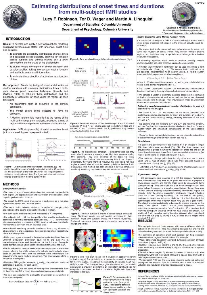
5. 1. 2. 3. Sustained. Transient. 3. 45-90 s. 4. 90-160 s. 5. 2. 4. HR. Cognitive & Affective Control Lab. Visual cue | Speech preparation. Onset of speech task. http://www.columbia.edu/cu/psychology/tor/. 1. * Download this poster at the website above. 528 T-PM.

E N D
5 1 2 3 Sustained Transient 3 45-90 s 4 90-160 s 5 2 4 HR Cognitive & Affective Control Lab Visual cue | Speech preparation Onset of speech task http://www.columbia.edu/cu/psychology/tor/ 1 * Download this poster at the website above 528 T-PM Estimating distributions of onset times and durations from multi-subject fMRI studies Lucy F. Robinson, Tor D. Wager and Martin A. Lindquist Department of Statistics, Columbia University Department of Psychology, Columbia University • Spatial Clustering using Markov Random Fields • A natural unit of analysis in fMRI is a multi-voxel region whose voxels show similar properties with respect to the timing of activation and de-activation. • We expect that similar voxels will tend to be grouped in space, but allow that clusters of similar voxels may contain multiple disjoint regions, and that there may be spatially abrupt changes in activation characteristics (edges). • A clustering algorithm which tends to produce spatially smooth clusters and also has edge-preserving properties is desirable. • A Hidden Markov Random field model can be used to estimate a field of cluster labels, . We assume that conditional on a pre-specified neighborhood Ni of nearby voxels, a voxel’s cluster membership is independent of all non-neighbors: • where denotes all labels except and are only labels from voxels in the defined neighborhood of . • The Markov assumption reduces the considerable computational burden in estimating the map of spatially dependent cluster labels. • We compile a vector of summary statistics based on the estimated activation characteristics of each voxel, and use this as our observed data in segmenting the image. Prior knowledge of image or anatomical characteristics can also be included. INTRODUCTION • Goals: To develop and apply a new approach for modeling sustained psychological states with uncertain onset time and duration. • To estimate the probability distributions of onset times and durations across subjects, allowing for variation across subjects and without making any a priori assumptions on the shape of the distributions. • To cluster voxels into regions of similar activation and duration profiles, taking into account spatial location and available anatomical information. • To estimate the probability of activation as a function of time. • Our approach: Treats the timing of onset and duration as random variables with unknown distributions. Uses a multi-path change point detection technique (Joseph and Wolfson, 1993) to estimate these distributions and the probability of activation for each voxel (or region) at each time point. • No parametric form is assumed in the density estimation. • The model allows some subjects to have no activation. • A Markov random field model is fit to the results of the multi-path change point analysis, producing a map of regions with homogeneous activation characteristics. • Application: fMRI study (n = 24) of social evaluative threat (a 2 min stressful speech-preparation task). Figure 2. True simulated image (left) and estimated clusters (right) A B Cluster 2 (light green) True pop. activation distribution (red) and estimated (blue) C D A B Cluster 3 (dark red) • Estimating population onset and duration distributions (g and g ) based on cluster analysis • For cluster k, k= 1….K, we assume that the voxels contained in a cluster have common distributions for onset and duration, g(k) and g(k), and that the voxel-specific ĝ and ĝ are noisy estimates of the true g(k)and g(k). • We assume that the functions g(k) and g(k) are relatively smooth, and use B-splines to compute estimated distribution functions for each cluster which are smoothed combinations of the voxel-specific estimates. • Based on these estimated distributions, we can compute probabilities of activation through time for each cluster, see Fig. 6. True pop. activation distribution (red) and estimated (blue) C D Figure 3. Results of analysis on simulated image - A and B show the estimated P and P for voxels assigned to clusters 2 (top) and 3 (bottom). C and D show the true P and P (red dotted line), and the smoothed estimates (blue line). • Simulations • To assess the performance of this method, 64 x 64 images of length 200 time points were simulated (Fig. 2A). The time courses are grouped into 3 groups in which the locations of shifts into and out of the activated state were drawn from drawn randomly from common (by region) distributions for onset and duration (Fig. 3). • The multi-path change point detection algorithm was run on each voxel, and a map of cluster labels was then assigned based on characteristics of the ĝand ĝ (Fig. 2B). • Estimates of g(k)and g(k) are computed using smoothing splines on the within-cluster estimates of g and g (Fig. 3C-D). • Experimental design • 24 participants were scanned in a 3T GE magnet. Participants were informed that they were to be given two minutes to prepare a seven-minute speech, and that the topic would be revealed to them during scanning. They were told that after the scanning session, they would deliver the speech to a panel of expert judges, though there was “a small chance” that they would be randomly selected not to give the speech. After the start of acquisition, participants viewed a fixation cross for 2 min (resting baseline). At the end of this period, participants viewed an instruction slide for 15 s that described the speech topic, which was to speak about “why you are a good friend.” The slide instructed participants to be sure to prepare enough for the entire 7 min period. After 2 min of silent preparation, another instruction screen appeared (a ‘relief’ instruction, 15 s duration) that informed participants that they would not have to give the speech. An additional 2 min period of resting baseline followed, which completed the functional run (Fig. 5). During a run, a series of 215 images were acquired (TR = 2s). Figure 4. The experimental paradigm - Participants were told they would silently prepare a speech under high time pressure during fMRI scanning. They were informed of the topic via visual presentation after 2 min of baseline scanning. After 2 min of speech preparation, they were informed (visually) that they would not have to give a speech after all, and they rested quietly for the final 2 min of scanning. This method has been effective in several samples at transiently increasing reported anxiety and autonomic arousal. Figure 1. (A) Simulated time courses for 10 subjects. (B) The distribution of the onset of activity estimated from the 10 subjects. (C) The distribution of the width of activity. (D) The probability of activation as a function of time. The figure indicates an increased chance of activation in the time period 40-80. METHODS • Change Point Analysis • We make no a priori assumptions about the nature of changes in the fMRI signal. Our approach can handle activation or deactivation, short or prolonged activation duration. • We model the fMRI signal time course in each voxel as a two-state system with “active” and “inactive” states. • The voxel shifts between states at a series of change points depending on the psycho-biological demands of the task. • For each voxel, we have data from M subjects at N time points. • For subject i, i=1 . . .M, the time profile of the voxel is modeled as a sequence of normally distributed observations yij , j=1 . . .N which may at an unknown time i undergo a shift in mean of unknown magnitude, representing a transition into an activated state. • An activated voxel may return to baseline at time i +i, where i is also unknown. i and i represent the onset and duration, respectively, of the activation profile. • Both i and i are assumed to be random variables drawn from an unknown population distribution (g(t)=P(i=t) and g(t)=P(i=t), respectively) which we seek to estimate. At the first level of analysis, these distributions are voxel-specific and can differ across the brain. • We fit a Gaussian mixture model with two components to each time course, allowing that shifts between the activate and inactivate states occur at unknown times, and that between shifts observations are drawn from the same mixture component. The time between shifts is treated as missing data. • Using the EM algorithm, we obtain ĝ and ĝ, the maximum likelihood estimates of g and g for each voxel. • Using ĝ and ĝ, we can compute voxel-specific characteristics such as the mean and SD of onset times and durations across subjects. • We can also calculate the probability of activation as a function of time across subjects: Figure 5. The brain surface is shown in lateral oblique and axial views. Significant voxels are color-coded according to their activation onset and duration (based on k-means clustering). Sustained responses during speech preparation are shown in orange and yellow. RESULTS • This analysis detected brain regions with several different kinds of activation time-courses. This was possible because the analysis did not make strong assumptions about the timing and duration of activity. • The estimates of activation onset and duration can help constrain inferences about regional brain function. For example: • Visual cortex was transiently activated during presentation of visual instructions (region 1 in Fig. 6). • Superior temporal sulci (regions 2 and 4), DLPFC, and other regions show moderately sustained activity during the initial 45 sec of speech preparation. • Ventral striatum (region 3) showed increases in activity only after participants were told they would not have to speak, consistent with a relief or positive emotional state. • Ventromedial PFC was the only area showing sustained activation throughout the stressor. This is consistent with a role in emotional valuation and regulation of autonomic responses to stress. Figure 6. (left) The brain is split into 5 clusters of spatially coherent activation. (right) The probability of activation is shown in a heat map for the five regions. In addition the probability of elevated heart rate (HR) is shown. The timing of the original visual cue and the speech preparation is shown in block format on the bottom right hand side for comparison purposes. Activation correlated highly with heart-rate increases in the task. REFERENCES Lindquist, Waugh & Wager (2007). Modeling state-related fMRI activity using change-point theory. NeuroImage, 35, 1125-1141. Lindquist & Wager. (2008) “Application of change-point theory to modeling state-related activity in fMRI”. In Pat Cohen (Ed), Applied Data Analytic Techniques for "Turning Points Research. Mahwah, NJ : Lawrence Erlbaum Associates Publishers. Joseph and Wolfson (1993) . “Maximum-likelihood estimation in th multi-path change-point problem.” Annals of the Institute of Statistical Mathematics 45(3) 511-530 Figure 7. Group-average time course (HEWMA) from medial prefrontal cortex (orange at right). The baseline period is shown in gray, and time points with significant activation are shown in red.