Download
1 / 42
420 likes | 550 Views
SPINOR Inversions based on RFs. Asymmetric profiles and ME (1). MHD-Simulations (Vögler et al. 2005). Asymmetric profiles and ME (2). MHD-Simulations (Vögler et al. 2005). Fe I 630.1 and 630.2 profiles degraded to SP pixel size.

E N D
Asymmetric profiles and ME (1) MHD-Simulations (Vögler et al. 2005)
Asymmetric profiles and ME (2) MHD-Simulations (Vögler et al. 2005) • Fe I 630.1 and 630.2 profilesdegradedto SP pixel size • Maps of inferred B and vLOSvery similar to real ones!
Inversions with gradients • Inversioncodescapable of dealingwithgradients • Are basedonnumericalsolution of RTE • Providereliablethermalinformation • Use less free parametersthan MEcodes (7 vs 8) • Inferstratifications of physicalparameterswithdepth • Produce betterfitstoasymmetric Stokes profiles • Heightdependence of atmosphericparametersisneededfor • easiersolution of the180o azimuthdisambiguity • 3D structure of sunspots and pores • Magnetic flux cancellationevents • Polarityinversionlines • Dynamicalstate of coronal loopfootpoints • wavepropagationanalysis • …
Example: SIR inversion Bellot Rubio et al. (2007) + • Spatial resolution: 0.4" • VIP + TESOS + KAOS • Inversion: SIR with 10 free parameters
Non-ME Inversion Codes SIR Ruiz Cobo& del Toro Iniesta (1992) 1C & 2C atmospheres, arbitrary stratifications, any photospheric line SIR/FT Bellot Rubio et al. (1996) Thin flux tube model, arbitrary stratifications, any photospheric line SIR/NLTE Socas-Navarro et al. (1998) NLTE line transfer, arbitrary stratifications SIR/GAUS Bellot Rubio (2003) Uncombed penumbral model, arbitrary stratifications SPINOR Frutiger & Solanki (2001) 1C & 2C (nC) atmospheres, arbitrary stratifications, any photospheric line, molecular lines, flux tube model, uncombed model LILIA Socas-Navarro (2001) 1C atmospheres, arbitrary stratifications MISMA IC Sánchez Almeida (1997) MISMA model, arbitrary stratifications, any photospheric line
SPINOR core: the synthesis • RTE has to be solved for • each spectral line • each line-of sight • each iteration efficient computation required! atmospheric parameters: T ... gas temperature B ... magn. field strength γ,φ ... incl. / azimuth angle of B vLOS ... line-of sight velocity vmic ... micro-turbulent velocity AX ... abundance (AH=12) G ... grav. acc. at surface vmac ... macro-turbulence vinst ... instr. broadening vabs ... abs. velocity Sun-Earth height / tau dependent height independent
Contribution Functions (1) The contribution function (CF) describes how different atmospheric layers contribute to the observed spectrum. Mathematical definition:CF ≡ integrand of formal sol. of RTE(here isotropic case, no B field): line core: highestformationwings: lowest formation Intuitively: profile shape indicates atmospheric opacity. Medium is more transparent (less heavily absorbed) in wings. one can see „deeper“ into the atmosphere at the wings.
Contribution functions (2) The general case: Height of formation: „This line is formed at x km above the reference, the other line is formed at y km …“ • caution with this statement is highly recommended! • CFs are strongly dependent on model atmosphere • different physical quantities are measured at different atmospheric heights
Response Functions „brute force method“: • synthesis of Stokes spectrum in given model atmosphere • perturbation of one atm. parameter • synthesis of „perturbed“ Stokes spectrum • calculation of ratio between both spectra • repeat (2)-(4) for all τi, λi, atm. parameter, atm. comp. The smart way: • knowledge of source function, evolution operator and propagation matrix direct computation of RFs possible (all parameters known from solution of RTE, simple derivatives)
Response functions Linearization: small perturbation in physical parameters of the model atmosphere propagate „linearly“ to small changes in the observed Stokes spectrum. introduce these modifications into RTE: only take 1st order terms, and introduce contribution function to perturbations of observed Stokes profiles response functions
Response Functions (2) RFs have the role of partial derivatives of the Stokes profiles with respect to the physical quantities of the model atmosphere: • In words:If xk is modified by a unit perturbation in a restricted neighborhood around τ0, then the values of Rk around τ0 give us the ensuing variation of the Stokes vector. • Response function units are inverse of their corresponding quantities (e.g RFs to temperature have units K-1)
RFs – Example: Fe 6302.5 Temp • model on the left is: • 500 K hotter • 500 G stronger • 20° more inclined • 50° larger azimuth • no VLOS gradient(right: linear gradient) |B| VLOS
SPINOR: Versatility Plane-parallel, 1-component models to obtain averaged properties of the atmosphere Multiple components (e.g. to take care of scattered light, or unresolved features on the Sun). Allows for arbitrary number of magnetic or field-free components (turns out to be important, e.g. in flare observations, where we have seen 4-5 components). Flux-tubes in total pressure equilibrium with surroundings, at arbitrary inclination in field-free (or weak-field surroundings) embedded in strong fields (e.g. sunspot penumbra, or umbral dots) includes the presence of multiple flux tubes along a ray when computing away from disk centre efficient computation of lines across jumps in atmospheric quantities Integration over solar or stellar disk, including solar/stellar rotation molecular lines (S. Berdyugina) non-LTE (MULTI 2.2, not tested yet, requires brave MULTI expert)
Penumbral Flux Tubes SPINOR applied to:Fe I 6301 + 6302Fe I 6303.5Ti I 6303.75 1st component:tube ray (discontinuity at boundary) 2nd component:surrounding ray Borrero et al. 2006
Hinode SOT: 10-11-2006 SPINOR & HINODE
1 magnetic component, 5 nodes SPINOR & HINODE
SPINOR & HINODE flux tube model
Penumbral Flux Tubes • Borrero et al. 2006 confirms uncombed model flux tube thickness 100-300 km
Multi Ray Flux Tube Frutiger (2000) multiple rays pressure balance broadening of flux tube
2-comp model Sunspot + molecular lines Mathew et al. 2003 SPINOR applied to:Fe I 15648 / 15652 1 magn. comp (6 nodes)1 straylight comp. molecular OH lines with OH without OH
Wilson Depression SPINOR applied to:Fe I 15648 / 15652 1 magn. comp (4 nodes)1 straylight comp. molecular OH lines Mathew et al. 2003 investigation of thermal-magnetic relation
oscillations observed in Stokes-Q ofFeI 15662 and 15665 calc. phase difference between Q-osc. time delay 2-C inversion with straylight: FT-component magn. background RF-calc: difference in formation height (velocity): ~20 km relate time delay to speed of various wave modes Penumbral Oscillations Bloomfield et al. [2007]
oscillations observed in Stokes-Q ofFeI 15662 and 15665 calc. phase difference between Q-osc. time delay 2-C inversion with straylight: FT-component magn. background RF-calc: difference in formation height (velocity): ~20 km relate time delay to speed of various wave modes Penumbral Oscillations Bloomfield et al. [2007]
oscillations observed in Stokes-Q ofFeI 15662 and 15665 calc. phase difference between Q-osc. time delay RF-calc: difference in formation height (velocity): ~20 km 2-C inversion with straylight: FT-component magn. background relate time delay to speed of various wave modes Penumbral Oscillations Bloomfield et al. [2007]
oscillations observed in Stokes-Q ofFeI 15662 and 15665 calc. phase difference between Q-osc. time delay 2-C inversion with straylight: FT-component magn. background RF-calc: difference in formation height (velocity): ~20 km relate time delay to speed of various wave modes Penumbral Oscillations best agreement for:fast-mode wavespropagating 50° to the vertical Bloomfield et al. [2007]
Analysis of Umbral Dots (1) Analysis of 51 umbral dots using SPINOR: 30 peripheral, 21 central UDs nodes in log(τ): -3,-2,-1,0(spline-interpolated) of interest:atomspheric stratification T(τ), B(τ), VLOS(τ) INC, AZI, VMIC, VMAC const. no straylight (extensive tests showed, that inversions did not improve significantly) Riethmüller et al., 2008
Analysis of Umbral Dots (2) Riethmüller et al., 2008 center of UD:
Analysis of Umbral Dots (3) atmospheric stratification retrieved in center (red) and the diffuse surrounding (blue) Riethmüller et al., 2008
Analysis of Umbral Dots (4) Vertical cut through UD Riethmüller et al., 2008
Analysis of Umbral Dots (5) Conclusions: inversion results are remarkably similar to simulations of Schüssler & Vögler (2006) UDs differ from their surrounding mainly in lower layers T higher by ~ 550 K B lower by ~ 500 G upflow ~ 800 m/s differences to V&S: field strength of DB is found to be depth dependent surrounding downflows are present, but not as strong and as narrow as in MHD (resolution?) Riethmüller et al., 2008
<Bz> = 200 G; Grid: 576 x 576 x 100 (10 km horiz. cell size) Brightness Magnetic field . Analysis of Hi-Res Simulations (forward calc.) Vögler & Schüssler
Pore simulation: brightening near the limb R. Cameron et al. =0.3 =0.5 =1 =0.7
G-Band (Fraunhofer): spectral range from 4295 to 4315 Å contains many temperature-sensitive molecular lines (CH) SPINOR: G-band spectrum synthesis 241 CH lines + 87 atomic lines For comparison with observations, we define as G-band intensity the integral of the spectrum obtained from the simulation data: [Shelyag, 2004]
SPINOR: Installation and first usage Download from http://www.mps.mpg.de/homes/laggGBSO download-section spinoruse invert and IR$soft
Exercise IVSPINOR installation and basic usage • install and run SPINOR • atomic data file, wavelength boundary file • use xinv interface • SPINOR in synthesis (STOPRO)-mode • 1st inversion:Hinode dataset of HeLIx+ • play with noise level / initial values / parameter range • change log(τ) scale • try to get the atmospheric stratification of an asymmetric profile • invert HeLIx+ synthetic profiles Examples: http://www.mps.mpg.de/homes/lagg Abisko 2009 spinor abisko_spinor.tgz unpack in spinor/inversions:cd spinor/inversions ; tar xfz abisko_spinor.tgz