Download
1 / 10
100 likes | 227 Views
,. Direct Inverse Modeling with Stream Functions Brouwer, G.K., July 16, 2007 Poster: Brouwer, G.K., W. Zijl , P. Fokker, TNO, the Netherlands. ,. Contents Intro: well measurements, processes, inversion Revival of stream function Direct inversion with the Double Constraint

E N D
, Direct Inverse Modeling with Stream Functions Brouwer, G.K., July 16, 2007 Poster: Brouwer, G.K., W. Zijl, P. Fokker, TNO, the Netherlands
, Contents Intro: well measurements, processes, inversion Revival of stream function Direct inversion with the Double Constraint Constraints (P,Q), (water cut) Example assimilating water cut measurements Conclusions Future work
, • Well data in an oil reservoir with water injection: • Pressure (t), or flow potential f (t) • Flow oil (t), or Qo (t) (flux), qo(t) (flux density) • Flow water (t) • Two dynamical processes with (very) different time scale: • Pressure propagation • displacement of the phases • Direct inversion model (Darcy): • k=vtot/(flow potential gradient) or:
, (qy=dy/dx=0) q1=-dy1/dy, q2=-dy2/dy df/dx=const k1 w1 w2 k2 l1 l2 (qy=dy/dx=0) qx=-dy/dy=const df/dx=/const k1 k2 w Finding k in flow direction: “k is hidden in f” Solve by requiring S(li/ki)=constant at all times (M=/1) l Finding k perpendicular to flow: An arrival time (y) problem !
, Stream function Mores streamlines Solving y: Implemented in MoReS: “prescribed boundary conditions”
, Double constraint (Wexler, 1985, medical application): pressure BC (wells) > guessed pressure fieldf(x,y) (MoReS pot. run) posterior perm field k (x,y) iterate prior permeability field k (x,y) flux BC (wells) > guessed flow field vx, vy or y(x,y) (MoReS flow run)
, Y=0.67 Y=1.00 prod3 cprod3 injector prod2 c = 0 cprod2 c = inf. cprod1 Y=0.00 Y=0.33 prod1 Constraining on P, Q: For each stream tube: j: porosity DS=Sbf-Swc V=volume
, Correcting on wells first arrival stream tube travel time by changing dy/ds Apply DC iterate
, LINE: “truth” Blue circles: assim. of fluxes and pressures Bluesquares: restored watercut
, • conclusions: • double constraint honours hard data • Water cut (+ saturation fronts from 4-D seismics) can be assimilated • methodology can be applied with any forward simulator • (pressures and velocities have to be available) • recommendations: • reformulation for 3-D • software development for 3D, multi- phase flow • (prototype 3-D available) • integrate with (extended) Kalman filter • explore DC for upscaling