Download
1 / 33
330 likes | 439 Views
Math 507, Lecture 8, Fall 2003. Poisson Random Variables and Variance. Poisson Random Variables. Motivation

E N D
Math 507, Lecture 8, Fall 2003 Poisson Random Variables and Variance
Poisson Random Variables • Motivation • As cloth comes off an industrial loom, it occasionally has noticeable flaws. Suppose that a particular loom, producing cloth at a fixed standard width, produces, on average, one such flaw per linear foot (based on past studies of the quality of fabric from the loom). This means that some feet have no flaws while others have one, two, three, or more. How can we build a model of the probability of getting k flaws in a particular foot of cloth? Math 507, Lecture 8, Poisson and Variance
Poisson Random Variables • One approach is to divide each foot into n thin strips, each of length 1/n, choosing n so large (that is, making the strips so thin), that the probability of getting two or more flaws in a strip is effectively zero. Thus we can now treat each strip as having either no flaws or one flaw. If the loom produces flaws whose location is independent all other flaws, then these n strips constitute n independent trials, each of which has the same probability of containing a flaw. Thus the number of flaws, X, in a particular foot is a binomial random variable. Math 507, Lecture 8, Poisson and Variance
Poisson Random Variables • Which binomial random variable is X? Clearly n=n (who could argue with that), but what is p? We know that E(X)=the average number of flaws in n strips=the average number of flaws in a foot=1. But we already have a theorem that says the expected value of a binomial random variable is np. Thus for our particular X, we have np=1, or p=1/n. That is, X~binomial(n,1/n). Math 507, Lecture 8, Poisson and Variance
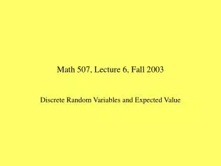
Poisson Random Variables • How large must n be to make the probability of two or more flaws in a strip effectively zero? The bigger the better! It might be interesting to look at the distribution of binomial(n,1/n) random variables as n increases in size. The following histogram shows the pdf of such random variables for n=2, 5, 7, 10, 100, and 1000. The bars for each n are distinguished by color, increasing from left to right. Math 507, Lecture 8, Poisson and Variance
Poisson Random Variables Math 507, Lecture 8, Poisson and Variance
Poisson Random Variables • Note the progression of the bars for each number of successes k. For k=0, 3, 4, 5 successes, the probability increases as n increases. For k=1,2 successes, the probability decreases as n increases. But in every case the difference between the bars for n=100 and n=1000 is tiny. There appears to be a limiting value as n increases. It turns out that this is correct. As n increases without limit, the probability of k successes approaches . (Note that by success we mean flaw, a somewhat perverse turn of phrase.) Math 507, Lecture 8, Poisson and Variance
Poisson Random Variables • The same intuition applies if the average number of flaws per linear foot of cloth, instead of being one, is some other number, say . If n is large enough, the probability of one flaw in a strip of length 1/n is /n and the number of flaws in one foot is binomial(n,/n). As n increases without limit, the probability of getting k successes (flaws) in one linear foot of cloth approaches (the result and proof are in Theorem 3.4 in the book). Math 507, Lecture 8, Poisson and Variance
Poisson Random Variables • Example: Suppose that a particular loom produces an average of 2.4 flaws per linear foot. What is the probability that the next foot we observe has exactly 3 flaws? Here =2.4 and k=3. So the probability is Math 507, Lecture 8, Poisson and Variance
Poisson Random Variables • Definition • It turns out that this formula has all the properties of a pdf. Thus we can use it to define a new random variable: We say that X is a Poisson random variable with parameter if X has pdf In this case we write X~Poisson(). Note that the range of X is the set of nonnegative integers, a countable infinite set, and so X is discrete. (Simeon Denis Poisson, 1781—1840, showed in 1837 how the Poisson is the limit of binomial probabilities, though de Moivre had done it in 1718). Math 507, Lecture 8, Poisson and Variance
Poisson Random Variables • The only pdf property that is not obvious in this definition is that we get a sum of 1 if we add up f(k) over all possible values of k. Here is the relevant calculation: Note that this depends on knowing the MacLaurin series for the exponential function, something every mathematician should know by heart! Math 507, Lecture 8, Poisson and Variance
Poisson Random Variables • Applications: Approximation to binomial distributions • Since the Poisson is the limit of particular binomial distributions, it seems reasonable that one could approximate binomial distributions with large n. This turns out to be correct. Surprisingly, though, the quality of the approximation depends much more on the value of p than that of n. Approximations are generally good if p is small and bad if it is not. A lovely demonstration of this lives at http://www.rfbarrow.btinternet.co.uk/htmasa2/Binomial1.htm. (It also demonstrates how the normal distribution approximates both the binomial and the Poisson. Math 507, Lecture 8, Poisson and Variance
Poisson Random Variables • Applications: Approximation to binomial distributions • Example: When leading computer manufacturer Gatepac ships a system, there is a 3% chance it will not work on arrival. If UT buys 200 new Gatepac systems, what is the probability that exactly 5 of them will not work? Let X be the number that fail. Then X~binomial(200,0.03). So Note that E(X)=200*0.03=6. Now let Y~Poisson(6). Then . The error is about 0.0016, but the second computation is much simpler if you have to do it by hand (use the MacLaurin series to approximate e^-6). Math 507, Lecture 8, Poisson and Variance
Poisson Random Variables • Poisson distributions in real life • Many phenomena in the Creation seem to follow a Poisson distribution. It was brought to the attention of the mathematical world by Ladislaus von Bortkiewicz in 1898 in a paper in which he used it to model the rate of deaths of Prussian soldiers by horse kicks (see http://www.hbcollege.com/business_stats/kohler/biographical_sketches/bio9.3.html). The general rule seems to be that Poisson distributions model the number of occurrences of events that occur uniformly (in some sense) but rather infrequently per small unit of time or space Math 507, Lecture 8, Poisson and Variance
Poisson Random Variables • Poisson distributions in real life • The book mentions other examples on p. 74: emission of radioactive particles in a fixed time, outbreaks of war in a fixed time, accidents in a fixed time, occurrence of stars in a fixed volume of space, misprints per page, flaws per unit area in an industrial process that produces sheets of some material. Math 507, Lecture 8, Poisson and Variance
Poisson Random Variables • Poisson distributions in real life: Example: • An average of 11 accidents per year happen at a particular intersection. What is the probability of two or more accidents happening there in a single day. Let X be the number of accidents there in a day. The average number of accidents in a day is 11/365, so X~Poisson(11/365). We want to find P(X>=2)=1-P(X<2)=1-f(0)-f(1). We see • That is, it should happen on average about every six years. Math 507, Lecture 8, Poisson and Variance
Poisson Random Variables • Expected Value: We have been treating as the expected value of a Poisson random variable, and this turns out to be correct. If X~Poisson(), then E(X)=. The theorem (3.5) and proof are in the book on pp. 73—74 . Math 507, Lecture 8, Poisson and Variance
Variance of Discrete Random Variables • Preliminary: Law Of The Unconscious Statistician (LOTUS) • If X is a discrete random variable on some sample space S and h is a real-valued function whose domain includes the range of X, then the composition h(X) is also a random variable on S. For example, if X is the roll of a die, and h(x)=(x-3)^2, then h(X) is a random variable with range {0,1,4,9}. Note that P(h(X)=0)=1/6, P(h(X)=1)=1/3, P(h(X)=4)=1/3, and P(h(X)=9)=1/6. Math 507, Lecture 8, Poisson and Variance
Variance of Discrete Random Variables • Preliminary: Law Of The Unconscious Statistician (LOTUS) • It turns out that there is a natural way to find the expected value of such a random variable. In fact it is so natural that it is hard to see that it is not the definition of expected value. Consider the random variable we just defined. By the definition of expected value E(h(X))=0*(1/6)+1*(1/3)+4*(1/3)+9*(1/6)=19/6. That is, we multiply every value of h(X) by its probability of happening and then sum the results. Math 507, Lecture 8, Poisson and Variance
Variance of Discrete Random Variables • Preliminary: Law Of The Unconscious Statistician (LOTUS) • It seems natural, however, just to go through all possible die rolls and multiply the value of h for that die roll by the probability of getting that roll. That is, Math 507, Lecture 8, Poisson and Variance
Variance of Discrete Random Variables • Preliminary: Law Of The Unconscious Statistician (LOTUS) • It is not a fluke that both approaches give the same result. It is a theorem (3.6) knows as the Law Of The Unconscious Statistician. Formally it says that if X is a discrete random variable with range , then That is, we can go through the possible values of X, apply h to them, multiply each result by the probability of getting that value of X, and then sum the products. This is often simpler than finding all the possible values of h(X) and their probabilities of occurring, as is necessary to use the definition of expected value of h(X) directly. Math 507, Lecture 8, Poisson and Variance
Variance of Discrete Random Variables • Corollaries to LOTUS • If X is a discrete random variable and a and b are real numbers, then E(aX+b)=aE(X)+b. (Theorem 3.7) • Example: Let X be the roll of a die. We know E(X)=7/2. Then E(5X-9)=5(7/2)-9=35/2 – 18/2=17/2. What does this mean? Suppose we play a game as follows: I roll a die and pay you $5 for every dot that comes up (e.g., I pay you $15 for a 3). You then pay me $9 for the privilege of playing the game. On average you will gain 17/2 dollars, that is $8.50, from every play of the game. Math 507, Lecture 8, Poisson and Variance
Variance of Discrete Random Variables • Corollaries to LOTUS • Note also Theorem 3.8 that says the expected value of a sum of functions of X equals the sum of the expected values of the functions applied to X individually. Math 507, Lecture 8, Poisson and Variance
Variance of Discrete Random Variables • Variance • The expected value is the “average” value of a random variable. Some random variables tend to take values close to their expected values, while others often take values far above or far below it. It is often helpful to have a measure of how far a random variable tends to be from its mean. This is sometimes called a measure of spread. The most common such measures are the variance and its square root, the standard deviation. • On pp. 76—77 the book discusses two natural measures of spread that fail to be very useful. The variance, on the other hand, seems a little less natural but is universally used. Math 507, Lecture 8, Poisson and Variance
Variance of Discrete Random Variables • Variance • Definition: If X is a discrete random variable, then the variance of X is defined by where is the expected value of X. That is, the variance is the expected squared deviation of X from its mean. We also denote it by . The square root of the variance is known as the standard deviation of X, denoted SD(X) or . Math 507, Lecture 8, Poisson and Variance
Variance of Discrete Random Variables • Variance • Example: Let X be the roll of a die. We know E(X)=1/6. Let us find Var(X). By definition of variance It follows immediately that Math 507, Lecture 8, Poisson and Variance
Variance of Discrete Random Variables • Variance • What do these numbers mean? Again they somehow measure how far away from the mean of 7/2 a die roll tends to be or how spread out the values of a die roll tend to be. We will be able to say more once we learn Chebyshev’s Theorem in section 3.10. • Theorem 3.9 gives us a simpler formula for finding the variance of a discrete random variable. Namely, Math 507, Lecture 8, Poisson and Variance
Variance of Discrete Random Variables • Variance • Example: Let us use the new formula to find Var(X) where X is a die roll. We already know By LOTUS we can compute So Math 507, Lecture 8, Poisson and Variance
Variance of Discrete Random Variables • Variance • Theorem 3.10 and its corollary: Let X be a random variable and a and b be real numbers. Then and These results are intuitive: If you shift X by b, its spread does not change. If you multiply X by a, then you change its spread by a factor of the magnitude of a (and thus the square of the spread by the square of a). Math 507, Lecture 8, Poisson and Variance
Variance of Discrete Random Variables • Variance • Example: Let X be the roll of a die. Suppose we play a game in which you roll a die and pay me twice the roll (in dollars) plus one dollar. What is the variance of this game? We want Math 507, Lecture 8, Poisson and Variance
Variance of Discrete Random Variables • Warning: Expected values and Variances need not exist if X has an infinite range. Math 507, Lecture 8, Poisson and Variance
Variance of Discrete Random Variables • The variance of the families of random variables we have met is easily calculated (see the book for the proofs) • If X~binomial(n,p), then Var(X)=npq • If X~geometric(p), then • If X~geometric(n,A,N), then Note that if we define p=A/n, then this formula becomes in which only the final factor differs from the variance of the binomial. Math 507, Lecture 8, Poisson and Variance
Variance of Discrete Random Variables • The variance of the families of random variables we have met is easily calculated (see the book for the proofs) • If X~Poisson(), then Var(X)=. Yes, Poisson random variables have the same expected value and variance. Math 507, Lecture 8, Poisson and Variance