Download
1 / 27
270 likes | 373 Views
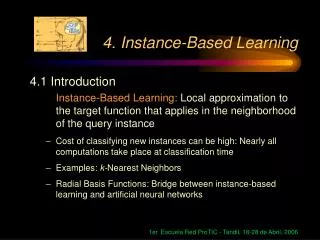
Instance-Based Learning. By Dong Xu State Key Lab of CAD&CG, ZJU. Overview. Learning Phase Simply store the presented training examples. Query Phase Retrieve similar related instances. Construct local approximation. Report the function value at query point.

E N D
Instance-Based Learning By Dong Xu State Key Lab of CAD&CG, ZJU
Overview • Learning Phase • Simply store the presented training examples. • Query Phase • Retrieve similar related instances. • Construct local approximation. • Report the function value at query point. Key Idea - Inference from neighbors(物以类聚)
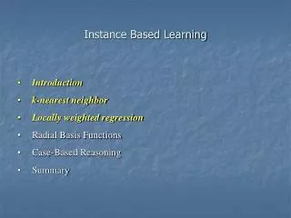
Perspective • Nearby instances is Related. (聚者必类) • Nearby (distance metric, distance is short) • Related (function value can be estimated from) • Distance Metric • Euclidean points • Feature Vector • Function Approximation • Lazy: k-Nearest Neighbor(kNN), Locally Weighted Regression, Case-Based Reasoning • Eager: Radial Basis Functions (RBFs) • In Essence, all methods are all local.
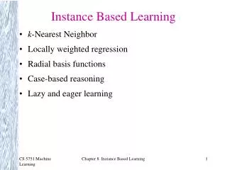
Three Methods • k-Nearest Neighbor • Discrete-valued functions (Voronoi diagram) • Continuous-valued functions (Distance-Weighted)
Three Methods • Locally Weighted Regression • Locally Weighted Linear Regression • Linear Approximation Function • Choose Weights by Energy Minimization
Three Methods • Radial Basis Functions • Target Function • Kernel Function • Two-Stage Learning Process • Learn the Kernel Function • Learn the Weights • They are trained separately. More efficient.
Remarks • How to decide the feature vectors so that avoid the “curse of dimensionality” problem? • Stretch the axes (weight each attribute differently, suppress the impact of irrelevant attributes). • Q: How to stretch? A: Cross-validation approach • Efficient Neighbor Searching • kd-tree (Bentley 1975, Friedman et al. 1977) • Q: How to decide k (# neighbors)? A: Can use range searching instead. • Kernel Function Selection • Constant, Linear, Quadratic, etc. • Weighting Function • Nearest, Constant, Linear, Inverse Square of Distance, Gaussian, etc. • Represent global target function as a linear combination of many local kernel functions (local approximations). • Query-Sensitive. Query phase may be time-consuming.
Have a rest, now come to our example.
Aaron Hertzmann et. al. SIGGRAPH 2001. : :: : A A’ B’ B Image Analogies Problem (“IMAGE ANALOGIES”): Given a pair of images A and A’ (the unfiltered and filtered source images, respectively), along with some additional unfiltered target image B, synthesize a new filtered target image B’ such that A : A’ :: B : B’
Questions • How to achieve “Image Analogies”? • How to choose the feature vector? • How many neighbors need to be consider? • How to avoid “curse of dimensionality”?
Outline • Relationships need to be described • Unfiltered image and its respective filtered image • The source pair and the target pair. • Feature Vector (Similarity Metric) • Based on an approximation of a Markov random field model. • Sample joint statistics of small neighborhoods within the image. • Using raw pixel value and, optionally, oriented derivative filters. • Algorithm • Multi-scale autoregression algorithm, based on previous texture synthesis methods [Wei and Lovey, 2000] and [Ashikhmin 2001]. • Applications
Feature Vector • Why RGB? • Intuitive, easy to implement. • Work for many examples. • Why luminance? • Can’t work for images with dramatic color differences. • Clever hack: luminance remapping. • Why steerable pyramid? • Still can’t work for line arts. • Need strengthen orientation information. • Acceleration • Feature Vector PCA (Dimension Reduction) • Search Strategies: ANN (Approximate Nearest Neighbor), TSVQ
Algorithm (1) • Initialization • Multi-scale (Gaussian pyramid) construction • Feature vector selection • Searching structure (kd-tree for ANN) build up • Data Structure • A(p): array p ∈ SourcePoint of Feature • A(p): array p ∈ SourcePoint of Feature • B(q): array q ∈ TargetPoint of Feature • B(q): array q ∈ TargetPoint of Feature • s(q): array q ∈ TargetPoint of SourcePoint
Algorithm (2) • Synthesis • function CREATEIMAGEANALOGY(A, A’, B): Compute Gaussian pyramids for A, A’, and B Compute features for A, A’, and B Initialize the search structures (e.g., for ANN) for each level l , from coarsest to finest, do: for each pixel q ∈ B’l, in scan-line order, do: p ← BESTMATCH(A, A’, B, B’, s, l , q) B’l(q) ← A’l(p) sl(q) ← p return B’l • function BESTMATCH(A, A’, B, B’, s, l , q): papp← BESTAPPROXIMATEMATCH(A, A’, B, B’, l , q) pcoh← BESTCOHERENCEMATCH(A, A’, B, B’, s, l , q) dapp← ||Fl(papp ) − Fl(q)||2 dcoh← ||Fl(pcoh) − Fl(q) ||2 if dcoh≤ dapp(1 + 2l−Lκ) then return pcoh else return papp κ- coherence parameter
Algorithm (3) • Best Approximate Match • The nearest pixel within the whole source image. • Search strategies: ANN, TSVQ. PCA (dimension reduction). • Best Coherence Match • Return best pixel that is coherent with some already-synthesized portion of B’l adjacent to q, which is the key insight of [Ashikhmin 2001].. • The BESTCOHERENCEMATCH procedure simply returns s(r*) +(q − r*), where r* = arg min r∈N(q) ||Fl(s(r) + (q − r)) − Fl(q)||2 and N(q) is the neighborhood of already synthesized pixels adjacent to q in B ’l.
Algorithm (4) Figure : Neighborhood Matching.
Algorithm (5) Figure : Coherent Matching
Applications (1) • Traditional image filters
Applications (2) • Improved texture synthesis
Applications (3) • Super-resolution
Applications (4) • Texture transfer
Applications (5) • Line arts
Applications (6) • Artistic filters
Applications (7) • Texture-by-numbers
Conclusion • Provide a very natural means of specifying image transformations. • A typical application of Instance-Based Learning • kNN approach. • DO NOT consider local reconstruction. Is this possible? • More analogies?
Resource • AutoRegression Analysis (AR) • http://astronomy.swin.edu.au/~pbourke/analysis/ar/ • Image Analogies Project Page • http://www.mrl.nyu.edu/projects/image-analogies/ • Reconstruction and Representation of 3D Objects with Radial Basis Functions • Carr et. al. SIGGRAPH 2001