Download
1 / 54
540 likes | 549 Views
Profiling of Relaxation Time and Diffusivity Distributions using Low Field NMR. Michael Rauschhuber George Hirasaki April 26, 2011. Motivation For NMR Profiling. Current NMR Profiling typically relies on slice selection multiple thin slices needed to generate a profile

E N D
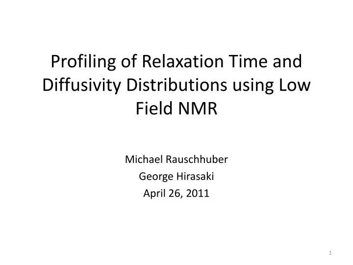
Profiling of Relaxation Time and Diffusivity Distributions using Low Field NMR Michael Rauschhuber George Hirasaki April 26, 2011
Motivation For NMR Profiling • Current NMR Profiling typically relies on slice selection • multiple thin slices needed to generate a profile • Saturation profiles can be determined only for air/water systems or D2O/oil systems. • Goal: Generation of profiles for oil/water systems without the need for multiple slice experiments.
Standard MRI technique to detect spatial information from a desired sample. In a uniform magnetic field, In the presence of a linear magnetic field gradient gx, Precession frequency is linearly related to spatial position Imaging Gradients x-xL Sample xcenter f-fL fL
Image Construction • Acquisition of the full echo is necessary for image construction. • Application of a FFT reconstruction is performed in order to generate the 1-D profile. • Finally, frequency can be converted to distance using the linear relationship between frequency and sample position.
Image Contrast for a Single Echo • Technique used to differentiate fluids with different T1 or T2.. • For Single Spin Echo Imaging Sequence, • By appropriately selecting TR and TE, spin density, T1-weighted, or T2-weighted images can be attained. TA: relaxation time of fast relaxing component TB: relaxation time of slow relaxing component For T1 Contrast, selection of TR should allow for one fluid to be fully polarized while the other is only partially polarized. Similarly, for T2 contrast, the proper choice of TE should allow for greater relaxation of one fluid than the other.
Spin Density ImageLayered Water – Squalane (C-30 oil, m = 22 cP) System TA= T2,squalane = 125 ms TB = T2,water = 2800 ms TE = 8 ms TE << TA < TB TR = 15000 ms TA < TB <<TR Squalane • Using a spin density image, the squalane and water layers cannot be differentiated from one another, because water and squalane have a similar Hydrogen Index. Water
T1-Weighted ImageLayered Water – Squalane System TA= T2,squalane = 125 ms TB = T2,water = 2800 ms TE = 8 ms TE << TA < TB TR = 714 ms TA <TR < TB Squalane • Due to the selection of TR, the squalane layer is fully polarized between scans while the water is only partially polarized. Therefore, the squalane layer has a greater amplitude in the image. Water
T2-Weighted ImageLayered Water – Squalane System TA= T2,squalane = 125 ms TB = T2,water = 2800 ms TE = 140 ms TA < TE < TB TR = 15000 ms TA < TB <<TR Squalane Water • Due to the selection of TE, the squalane layer has undergone much more relaxation than the water layer. Therefore, the water layer has a greater amplitude in the image.
t t t 2t p/2 p p p … RF D1 d2 d2 d1 g1 g2 g2 … Gradient … Signal Restriction: 2d1g1 = d2g2 TR >>TE T2 Profiling • A CPMG-style imagining sequence, known as Rapid Acquisition with Relaxation Enhancement (RARE), can be used to generate a collection of profiles with increasing T2 relaxation. • Spatial distribution of T2 can be achieved by analyzing the decay of the acquired profiles.
T2 Profiles Sample: Water, g1 = g2 = 0.800 G cm-1,d1 = 1.30 msec, t = 3.00 msec, DW = 40.0 msec, SI = 64
Yates Core Sample (D) Sample: Yates D, g1 = g2 = 0.800 G cm-1,d1 = 1.30 msec, t = 3.00 msec, DW = 80.0 msec, SI = 32
Texas Cream Limestone (TCL 80) Sample: TCL 80, g1 = g2 = 0.800 G cm-1,d1 = 1.30 msec, t = 3.00 msec, DW = 80.0 msec, SI = 32
NMR D-T2 Profiling • T2 can be spatially resolved using the RARE pulse sequence. • By incorporating diffusion gradient pulses, NMR imaging techniques allow for the measurement of fluid self-diffusion coefficients. • Simultaneous spatial resolution of D and T2 will allow for the determination of saturation profiles even when oil and water phase exhibit overlapping T2 distributions.
D’ tL tL tL tS tS tS tL d3 RF d3 d2 2d2 2d2 gD gD gF gF d1 gF Gradient d1 gD gD Signal Prephasing Gradient Readout Gradient Diffusion Gradients D-T2 Profiling Pulse Sequence
Saturation profiles can be determined for samples exhibiting overlapping T2 peaks for water and oil by utilizing the difference in diffusivity to distinguish their signals. Saturation Profiles • D-T2 maps were acquired in 3 cm segments and then were stacked together creating a composite image for the entire 1 ft. sand column. • Dwell Time (DW) was selected based on the detection length of the probe to prevent aliasing
Sandpack Experiments • Sandpack (U.S. Silica 20/40) • Porosity = 0.36 • Permeability = 80 Darcy • Initial Waterflood • Oilflood • Detection of Capillary End Effect • 0.3 PV Waterflood • 0.6 PV Waterflood
Water Saturated SandPack S0,mass = 0.00 S0,prof = 0.00 Saturation Profile of a water saturated sandpack
Identification of Capillary end effect S0,mass = 0.87 S0,prof = 0.86 Capillary end effect number NC,end = 0.81 Saturation Profile of oilflood. Capillary end effect can be identified at the top (outflow) end of the profile.
Oil Flood S0,mass = 0.88 S0,prof = 0.94 Capillary end effect number NC,end = 0.10 Saturation Profile of oilflood. Increasing inject rate from 5 ft day to 40 ft day helped in removing the end effect
0.3 PV Waterflood S0,mass = 0.63 S0,prof = 0.62 Mobility Ratio M = 1.2 Gravity Number NGrav = 0.93 Saturation Profile of a sandpack after 0.3 PV waterflood.
0.6 PV Waterflood S0,mass = 0.36 S0,prof = 0.35 Mobility Ratio M = 1.2 Gravity Number NGrav = 0.93 Saturation Profile of a sandpack after 0.6 PV waterflood.
Summary of Sandpack Saturation Profiles • Displacement of oil by water can by visualized through the generation of NMR saturation profiles. • After 0.3 PV waterflood, the water front advanced near the center of the column • After 0.6PV waterflood, breakthrough of water occurred, and the saturation profile confirms that the oil saturation near the outlet is below the initial oil saturation.
Conclusions • Two NMR profiling pulse sequences have been designed and implemented for the measurement of T2 and D-T2 in a low-field spectrometer. • 1-D NMR profiling allows for the detection of spatially varying properties, such as saturation and porosity, within a sample. • D-T2 profiling allows for the detection of two NMR sensitive phase when they possess a significant contrast in viscosities. • NMR determined saturation profiles extracted from D-T2 profiling results yielded profiles with averages very close to the average saturations determined via mass balance at various stages within the flooding process.
Backup Slides T2 Profiling
Backup Slides Selection of Imaging Parameters
Parameter Selection • Experimental parameters, such as sample size, gradient strength and duration, and the number and spacing of the acquired data points, must be selected to ensure that useful information can be extracted from the profiles • Attenuation due to diffusion is dependent on the product of gradient strength (g) and duration (d). Therefore, g and d should be selected in order to reduce the amount of the relaxation due to diffusion • The dwell time (DW), or spacing between acquired data points, determines the image length, and the number of data points collected per echo (SI) sets the number of points resolved over that distance.
Sample Size An FID of water, with a sample height of 0.5 cm, was performed at incremental locations within the probe to determine the sweet spot. • Sample should be located within the sweet spot of the NMR and centered about fL. Our MARAN has sweet spot of about 5 cm, so a sample with a height of 4 cm is used.
Effect of Diffusion For g1 = g2 = g and 2d1 = d2, where n is the echo number
Effect of Diffusion • Due to the presence of several gradient pulses, attenuation due to diffusion can be significant. As the product of gradient strength (g) and duration (d1) is increased, the effect of diffusion becomes more pronounced. For g1 = g2 = g and 2d1 = d2, where T2# is the apparent spin-spin relaxation time measured via RARE • Excessive attenuation due to diffusion is not desirable.
Minimum Gradient Strength • Attenuation due to diffusion is dependent on the product of g and d1. Therefore, weak gradients can be used to minimize this effect. • The gradient strength (g) deviates from the expected behavior at very low values. The lowest reliable gradient for the Maran-M was selected to be g = 0.8 G cm-1 which corresponds to the lowest gradient with less than 5% deviation between observed and predicted values.
Maximum Gradient Strength • The application of larger imaging gradients results in a larger range of frequencies encoded by the imaging pulses. • Profile rounding can occur when the range of encoded frequencies, Δf, takes up a large portion of the probe’s bandwidth. • The maximum gradient strength should be selected to prevent significant rounding of the profile due to bandwidth limitations.
Dwell Time (DW) • Dwell Time (DW) refers to the spacing between data points and sets the range of frequencies to be resolved by the measurement. DW must be selected in order to prevent aliasing of the signal using the Nyquist Criterion.
Number of Acquisition Points (SI) • The number of acquisition points (SI) corresponds to the number of data points collected per echo as well as the number of points across the profile. Selection of SI and DW determine the profile’s resolution • If data is acquired during the entire duration of the readout pulse, SI can be represented as
Selection Criteria T2#/T2 = 0.95 Resulting g and d1 pair: g = 0.80 G cm-1 d1 = 1.43 msec • Based on the sample size, the minimum T2 to be measured, and a selected value of T2#/T2 , a g and d1 pair can be chosen. • The largest possible d1 will allow for the longest echo train and subsequently, the broadest resolution of relaxation times.
Selection Criteria (cont’d). SI = 64 DW = 44 msec • Once a g and d1 pair has been choose, DW and SI can be selected. • Data must be acquired under the readout gradient. If we require data collection to last as long as possible, DW to be less than DWmax, and SI = 2n, then DW and SI can be determined.
D’ tL tL tL tS tS tS tL d3 RF d3 d2 2d2 2d2 gD gD gF gF d1 gF Gradient d1 gD gD Signal Prephasing Gradient Readout Gradient Diffusion Gradients Reducing Phase Sensitivity • Prepare magnetization with diffusion weighting first (Norris et al., 1992). • Introduce p/2 pulse during formation of first echo to remove out of phase signal (Alsop, 1997).
Unipolar vs. Bipolar 1st Experiment 4th Experiment Unipolar Bipolar
D’ tL tL tL tS tS tS tL d3 RF d3 d2 2d2 2d2 gD gD gF gF d1 gF Gradient d1 gD gD Signal Prephasing Gradient Readout Gradient Diffusion Gradients Reducing Phase Sensitivity • Prepare magnetization with diffusion weighting first (Norris et al., 1992). • Introduce p/2 pulse during formation of first echo to remove out of phase signal (Alsop, 1997).
Reducing Phase Sensitivity Prior to Modification After Modification Squalane, g = 2.5 G cm-1, d = 6 msec, h = 1.38 cm
Gradient Pre-pulses • Gradient pre-pulses allow for the consistent application of gradient pulses during the NMR experiment by warming up the gradient coils • Pre-pulses also add additional stability to the gradient waveform by balancing the effect of eddy currents on the system’s magnetization throughout the duration of the pulse sequence
Echo Shape in the Absence of Pre-pulses High g Low g One Peak Two Peaks • Examination of the echo data for the experiment shows that at low g values an echo with a single peak forms while the use of high g values results in echoes with two distinct peaks • Formation of dual peaks is indicative of a sequence in which the gradients prior to refocusing are not properly balanced by the gradients after refocusing. In other words, the magnitude and duration of the first set of bipolar pulses is not equivalent to the second set even though their parameters are identical
Effect of Pre-Pulses on Profile Shape 0 Pre-pulses 1 Pre-pulses 5 Pre-pulses 3 Pre-pulses 9 Pre-pulses 7 Pre-pulses • Profiles of first echo at g = 19.4, 27.2, 32.2, 38.0, and 45.0 G cm-1 for sandpack at initial oil saturation (SMY, water). The number of gradient pre-pulses varied between 0 and 9. • Profiles generated using too few pre-pulses demonstrate large variations and often times overlap with one another. As the number of pre-pulses was increased, the profiles start to flatten out and separate .
Effect of Pre-Pulses on Echo Shape 9 Pre-pulses 0 Pre-pulses Two Peaks One Peak • In the absence of gradient pre-pulses, two peaks were noted in the echo. This resulted in the large fluctuations in profile amplitude. • Gradient pre-pulses prevent the echo from forming two distinct peaks. This results in the profiles beginning to flatten out and separate.
Impact of Pre-pulses on the D-T2 Profile • In the absence of gradient pre-pulses, poorly shaped profiles manifest themselves as valleys in each region of interest in the intensity of the D data • Incorporating an adequate number of pre-pulses into the D-T2 profiling pulse sequences removes these valleys noted in projected D data. 9 Pre-pulses 0 Pre-pulses
Gradient-RF Pulse Spacing • If the spacing between RF and gradient pulses is less than the gradient fall time, then the two will overlap causing degradation of the NMR signal. • A series of FID experiments preceded by a gradient pulse can be used to examine the impact of RF-gradient spacing. • As the time between RF and gradient pulses increases, the FID decays more slowly indicating less impact of the gradient on the RF pulse. RF d3 gD d1 Gradient Signal FID performed after application of gradient pulse (g = 20.0 G cm-1 , d = 5.0 msec).
Selecting a Gradient-RF Pulse Spacing • FID results indicate that a spacing of 10 to 15 msec is needed to prevent the gradient from interacting with the RF. • With a gradient-RF spacing of 10 msec for the D-T2 profiling experiment, a large portion of the oil signal will be lost due to relaxation before the collection of the first echo. • In an effort to balance the NMR signal quality with the NMR signal strength, it is desired to collect the first echo before t = T2,logmean of the crude oil. Subsequently, gradient-RF spacing in the D-T2 profiling sequence was set to 5 msec. • Even at sub-optimum gradient-RF spacing, improvements are noted in the profile shape. Profile of 1st echo from D-T2 profiling sequence with g =19.4 G cm-1. Gradient-RF spacing is increased from 1.0 msec to 5.0 msec, and rounding behavior noted in profile is alleviated
Impact of Gradient-RF Pulse Spacing on Saturation Profiles 1 msec 5 msec Increasing the RF-gradient spacing helps to remove dips in the saturation profile. Consistent dip in saturation profile at the bottom of each measurement region when an insufficient gradient-RF spacing is applied
Backup Slides Data Processing: Rotating FFT Data to Generate a Meaningful Profile
Profile Rotation • FFT reconstruction of echo data yields both real and imaginary contribution to the profile. • FFT data for all echoes at a given height/frequency is rotated in order to generate 1-D profile.