Download
1 / 8
80 likes | 266 Views
The Adaline Neuron. Ranga Rodrigo February 8, 2014. Introduction. In the last lecture, we studied about the perceptron .

E N D
The Adaline Neuron Ranga Rodrigo February 8, 2014
Introduction • In the last lecture, we studied about the perceptron. • By minimizing the sum-of-squares error with respect to the weights, with the assumption of an identity activation function, we derived the Widrow-Hoff Learning Rule. • We implemented this in Matlab to carry out linear classification in 2 dimensions. • What we have implemented, actually, is the adaline model. • Today we consider more such models.
Adaline Neuron • The construction of this neuron is very similar to the perceptron model, and the only difference relates to the learning algorithm. • Computation of output signal y is identical to the perceptron. • However, the output desired signal d is compared to signal s at the output of the linear part of the neuron (adder).
Adaline Neuron x0 = 1 w0 x1 w1 w2 x2 s y x3 w3 wD xD - + d
% Adaline Neuron % Ranga Rodrigo % February 17, 2014 clc; clear all; close all c1 = [2,4; 3, 3]; c2 = [4, 8; 8, 4]; scatter(c1(:,1), c1(:,2), 'o', 'MarkerEdgeColor', 'b', 'MarkerFaceColor', [0, 0.5, 1]) hold on scatter(c2(:,1), c2(:,2), 'o', 'MarkerEdgeColor', 'r', 'MarkerFaceColor', [1, 0.5, 0.5]) axis([0,10, 0,10]) hold on eta = 0.02; % Learning rate (must be carefully selected) w = [-1, 4, 3]'; % Randomly initialize [w(1), w(2), theta] x = [c1; c2]; n = size(x,1); t = [ones(size(c1,1), 1); -ones(size(c2,1), 1)];
e = inf; k = 1; % Maximum number of iterations kmax = 1000; while e > 1 && k < kmax e = 0; for i = 1:n s = w'*[x(i,:), 1]' delta = (t(i) - s) w = w + eta*delta*[x(i, :), 1]' e = e + delta^2 end e k = k +1; % Plotting the current decision boundary p1 = [0, -w(3)/w(2)]'; p2 = [-w(3)/w(1), 0]'; line([p1(1), p2(1)], [p1(2), p2(2)]) pause(0.5) end
% Plotting the final decision boundary p1 = [0, -w(3)/w(2)]'; p2 = [-w(3)/w(1), 0]'; line([p1(1), p2(1)], [p1(2), p2(2)], 'Color', 'm', 'LineWidth', 4) % Test point x = [2,1]'; y = stepfun(w'*[x', 1]'); if y == 1 scatter(x(1), x(2), 's', 'MarkerEdgeColor', 'b', 'MarkerFaceColor', [0, 0.5, 1]) else scatter(x(1), x(2), 's', 'MarkerEdgeColor', 'r', 'MarkerFaceColor', [1, 0.5, 0.5]) end