Download
1 / 45
450 likes | 585 Views
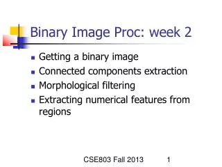
Binary Image Proc: week 2. Getting a binary image Connected components extraction Morphological filtering Extracting numerical features from regions. Quick look at thresholding. Separate objects from background. 2 class or many class problem? How to do it? Discuss methods later.

E N D
Binary Image Proc: week 2 • Getting a binary image • Connected components extraction • Morphological filtering • Extracting numerical features from regions Stockman CSE803 Fall 2008
Quick look at thresholding • Separate objects from background. • 2 class or many class problem? • How to do it? • Discuss methods later. Stockman CSE803 Fall 2008
Cherry image shows 3 regions • Background is black • Healthy cherry is bright • Bruise is medium dark • Histogram shows two cherry regions (black background has been removed) Use this gray value to separate Stockman CSE803 Fall 2008
Choosing a threshold • Common to find the deepest valley between two modes of bimodal histogram • Or, can level-slice using the intensities values a and b that bracket the mode of the desired objects • Can fit two or more Gaussian curves to the histogram • Can do optimization on above (Ohta et al) Stockman CSE803 Fall 2008
Connected components • Assume thresholding obtained binary image • Aggregate pixels of each object • 2 different program controls • Different uses of data structures • Related to paint/search algs • Compute features from each object region Stockman CSE803 Fall 2008
Notes on Binary Image Proc • Connected Components Algorithms • Separate objects from background • Aggregate pixels for each object • Compute features for each object • Different ways of program control • Different uses of data structures • Related to paint/search algs Stockman CSE803 Fall 2008
Example red blood cell image • Many blood cells are separate objects • Many touch – bad! • Salt and pepper noise from thresholding • How useable is this data? Stockman CSE803 Fall 2008
Cleaning up thresholding results • Can delete object pixels on boundary to better separate parts. • Can fill small holes • Can delete tiny objects • (last 2 are “salt-and-pepper” noise) Stockman CSE803 Fall 2008
Removing salt-and-pepper • Change pixels all of whose neighbors are different (coercion!): see hole filled at right • Delete objects that are tiny relative to targets: see some islands removed at right Stockman CSE803 Fall 2008
Simple morphological cleanup • Can be done just after thresholding -- remove salt and pepper • Can be done after connected components are extracted -- discard regions that are too small or too large to be the target Stockman CSE803 Fall 2008
CC analysis of red blood cells • 63 separate objects detected • Single cells have area about 50 • Noise spots • Gobs of cells Stockman CSE803 Fall 2008
More control of imaging • More uniform objects • More uniform background • Thresholding works • Objects actually separated Stockman CSE803 Fall 2008
Results of “pacmen” analysis • 15 objects detected • Location known • Area known • 3 distinct clusters of 5 values of area; 85, 145, 293 Stockman CSE803 Fall 2008
Results of “coloring” objects • Each object is a connected set of pixels • Object label is “color” • How is this done? Stockman CSE803 Fall 2008
Extracting components: Alg A • Collect connected foreground pixels into separate objects – label pixels with same color • A) collect by “random access” of pixels using “paint” or “fill” algorithm Stockman CSE803 Fall 2008
paint/fill algorithm • Obj region must be bounded by background • Start at any pixel [r,c] inside obj • Recursively color neighbors Stockman CSE803 Fall 2008
Events of paint/fill algorithm • PP denotes “processing point” • If PP outside image, return to prior PP • If PP already labeled, return to prior PP • If PP is backgr. pixel, return to prior PP • If PP is unlabeled obj pixel, then 1) label PP with current color code 2) recursively label neighbors N1, …, N8 (or N1, …, N4) Stockman CSE803 Fall 2008
Color closed boundary with L Choose pixel [r,c] inside boundary Call FILL FILL ( I, r, c, L) If [r,c] is out, return If I[r,c] == L, return I[r,c] L // color it For all neighbors [rn,cn] FILL(I, rn, cn, L) Recursive Paint/Fill Alg: 1 region Stockman CSE803 Fall 2008
Connected components using recursive Paint/Fill • Raster scan until object pixel found • Assign new color for new object • Search through all connected neighbors until the entire object is labeled • Return to the raster scan to search for another object pixel Stockman CSE803 Fall 2008
Extracting 5 objects Stockman CSE803 Fall 2008
Outside material to cover • Look at C++ functions for raster scanning and pixel “propagation” • Study related fill algorithm • Discuss how the recursion works • Prove that all pixels connected to the start pixel must be colored the same Stockman CSE803 Fall 2008
Alg B: raster scan control Visit each image pixel once, going by row and then column. Propagate color to neighbors below and to the right. Keep track of merging colors. Stockman CSE803 Fall 2008
Raster scanning control Stockman CSE803 Fall 2008
Events controlled by neighbors • If all Ni background, then PP gets new color code • If all Ni same color L, then PP gets L • If Ni != Nj, then take smallest code and “make” all same • See Ch 3.4 of S&S Stockman CSE803 Fall 2008
Merging connecting regions Detect and record merges while raster scanning. Use equivalence table to recode Stockman CSE803 Fall 2008
Visits pixels more than once Needs full image Recursion or stacking slower than B No need to recolor Can compute features on the fly Can quit if search object found (tracking?) “visits” each pixel once Needs only 2 rows of image at a time Need to merge colors and region features when regions merge Typically faster Not suited for heuristic start pixel alg A versus alg B Stockman CSE803 Fall 2008
Outside material • More examples of raster scanning • Union-find algorithm and parent table • Computing features from labeled object region • More on recursion and C++ Stockman CSE803 Fall 2008
Computing features of regions Can postprocess results of CC alg. Or, can compute as pixels are aggregated Stockman CSE803 Fall 2008
Area and centroid Stockman CSE803 Fall 2008
Second moments These are invariant to object location in the image. Stockman CSE803 Fall 2008
Contrast second moments • For the letter ‘I’ • Versus the letter ‘O’ • Versus the underline ‘_’ r c Stockman CSE803 Fall 2008
Perimeter pixels and length Stockman CSE803 Fall 2008
Circularity or elongation Stockman CSE803 Fall 2008
Circularity as variance of “radius” Stockman CSE803 Fall 2008
Radial mass transform • for each radius r, accumulate the mass at distance r from the centroid (rotation and translation invariant) • can iterate over bounding box and for each pixel, compute a rounded r and increment histogram of mass H[r] Stockman CSE803 Fall 2008
Interest point detection • Centroids of regions can be interesting points for analysis and matching. • What do we do if regions are difficult to extract? • We might transform an image neighborhood into a feature vector, and then classify as “interesting” vs “not”. Stockman CSE803 Fall 2008
Slice of spine MRI and interesting points selected by RMT & SVM Stockman CSE803 Fall 2008
3D microvolumes from Argonne high energy sensor: 1 micron voxels Ram CAT slice of a bee stinger (left) versus segmented slice (right). Each voxel is about 2 microns per side. Stockman CSE803 Fall 2008
Scanning technique used CCD camera material sample X-rays scintillator Pin head X-rays partly absorbed by sample; excite scintillator producing image in the camera; rotate sample a few degrees and produce another image; 3D reconstruction using CT rotate Stockman CSE803 Fall 2008
Different view of stinger Rendered using ray tracing and pseudo coloring based on the material density clusters that were used to separate object from background. (Data scanned at Argonne National Labs) Stockman CSE803 Fall 2008
Section of interesting points from RMT&SVM Stockman CSE803 Fall 2008
Segmentation of Scutigera Stockman CSE803 Fall 2008
Scutergera: a tiny crustacean • organism is smaller than • 1 mm • scanned by • volume segmented and • meshed by Paul Albee • roughly ten million triangles • to represent the surface • anaglyph created for 3D • visualization (view with glasses) Stockman CSE803 Fall 2008
Axis of least inertia • gives object oriented coordinate system • passes through centroid • axis of most inertia is perpendicular to it • concept extends to 3D and nD Stockman CSE803 Fall 2008
Derive the formula for best axis • use least squares to derive the tangent angle q of the axis of least inertia • express tan 2q in terms of the 3 second moments • interpret the formula for a circle of pixels and a straight line of pixels Stockman CSE803 Fall 2008