Download
1 / 16
160 likes | 260 Views
Components of Scientific Programming. Definition of problem Physical/mathematical formulation ( Focus today ) Development of computer code ( Focus to date ) Development of logic (e.g., flowchart) Assembly of correct lines of code Testing and troubleshooting Visualization of results

E N D
Components of Scientific Programming • Definition of problem • Physical/mathematical formulation (Focus today) • Development of computer code (Focus to date) • Development of logic (e.g., flowchart) • Assembly of correct lines of code • Testing and troubleshooting • Visualization of results • Optimization of code • Analysis of results • Synthesis
Steady-State Heat Conduction Equation Qin Qout dx In this exercise, no major Matlab concepts need to be implemented. The focus is on a small change in the coding and mathematics as a result of the physics extending from 1-D to 2-D.
Steady-State Heat Conduction Equation (1-D) Qin Qout Insulated wire or rod dx Change in thermal energy in time = Heat flow out - Heat-flow in T = temperature, and x = position We will represent dT/dx as T'. At steady state, the rate of energy change (E*) is zero:
Steady-State Heat Conduction Equation (1-D) Qin Qout dx At steady state,the rate of energy change (E*) is zero everywhere, so E* does not change as a function of position (x): This is the Laplace equation, one of the most important equations in physics
What does T" = 0 mean? • T' = constant • A plot of T vs. x must be a line. • T must vary linearly between any two points along the rod at steady state. • If T is known at positions xi-1 and xi+1, then T(i) = [T(i-1) + T(i+1) ]/2 • T(i) = average of Tat the nearby equidistant points (see Appendix for more detail) xi-2 xi-1 xi xi+1 xi+2
1-D Steady State Heat Conduction (a) num_iterations = 500; x = 1:50; T = 10.*rand(size(x)); % initial temperature distribution n = length(x); for j = 1:num_iterations % a "for loop" is used here for i=2:n-1; % Don't change T at the ends of the rod! T(i) = (T(i+1) + T(i-1))./2; end figure(1); clf; plot(x,T); axis([0 n 0 10]); xlabel('x'); ylabel('T'); end Interior Pt. Boundary Pt. with fixed boundary conditions Boundary Pt. with fixed boundary conditions x1 x2 xi x49 x50 i =1 i = 2 i = i i = 49 i = 50
1-D Steady State Heat Conduction (b) num_iterations = 500; x = 1:50; T = 10.*rand(size(x)); % initial temperature distribution n = length(x); for j = 1:num_iterations % a "for loop" is used here T(2:n-1) = (T (3:n) + T(1:n-2))./2; figure(1); clf; plot(x,T); axis([0 n 0 10]); xlabel('x'); ylabel('T'); end % Shorter, and it runs, but it introduces “noise” Interior Pt. Interior Pt. Boundary Pt. with fixed boundary conditions Boundary Pt. with fixed boundary conditions x1 x2 xi x49 x50 i =1 i = 2 i = i i = 49 i = 50
1-D Steady State Heat Conduction (c) x = 1:50; T = 10.*rand(size(x)); % initial temperature distribution n = length(x); tol = 0.1; dT = tol.*2.*ones(size(T)); % Initialize dT while max(abs(dT)) > tol % a "while loop" is used here for i=2:n-1 ; dT(i) = ((T(i+1) + T(i-1))./2) -T(i); % Change in T T(i) = T(i) + dT(i); % New T = old T + change in T end figure(1); clf; plot(x,T); axis([0 n 0 10]);figure(2) ; plot(x,dT); end % Hit ctrl-c to stop. Why won’t this stop? Interior Pt. Boundary Pt. with fixed boundary conditions Boundary Pt. with fixed boundary conditions x1 x2 xi x49 x50 i =1 i = 2 i = i i = 49 i = 50
1-D Steady State Heat Conduction (d) x = 1:50; T = 10.*rand(size(x)); % intial temperature distribution n = length(x); tol = 0.0001; dT = tol.*2.*ones(size(T)); % Initialize dT while max(abs(dT(2:n-1))) > tol % a "while loop" is used here for i=2:n-1 ; dT(i) = ((T(i+1) + T(i-1))./2) -T(i); % Change in T T(i) = T(i) + dT(i); % New T = old T + change in T end figure(1); clf; plot(x,T); axis([0 n 0 10]); xlabel('x'); ylabel('T'); end Interior Pt. Boundary Pt. with boundary conditions Boundary Pt. with boundary conditions x1 x2 x3 x4 x5 i =1 i = 2 i = 3 i = 4 i = 5
2-D Steady State Heat Conduction Equation For a 2-D problem, the temperature at a point is the average of T at the four nearest neighbors Boundary Condition (fixed) y5 y4 y3 y2 y1 Interior Point Note: grid is square Dx = Dy x1 x2 x3 x4 x5 x6 x7 x8 x9
2-D Steady State Heat Conduction Equation *Add a loop to account for 2-D grid *Reformulate T(xi) to account for 2-D *Check for convergence Boundary Condition (fixed) y5 y4 y3 y2 y1 Interior Point Note: grid is square Dx = Dy x1 x2 x3 x4 x5 x6 x7 x8 x9
Appendix • This appendix shows in more detail how the second derivative d2T/dx2 is evaluated numerically using a finite difference approximation method.
Solution of 1-D Steady State Heat Conduction Equation x-x x+(Dx)/2 x x+(Dx)/2 x+Dx
1-D Steady State Heat Conduction Equation x-2Dx x+Dx x x+Dx x+2Dx
1-D Steady State Heat Conduction Equation In words, what does this mean? xi-2 xi-1 xi xi+1 xi+2