Download

1 / 17
170 likes | 299 Views
Overview Examples of Supply Chain Management Problems Some Computer Science Preliminaries Exact Algorithms Structural Properties of Local Search Algorithms for the TSP Node Swapping Algorithms for the TSP Conclusions. Examples of Supply Chain Management Problems

E N D
Overview Examples of Supply Chain Management Problems Some Computer Science Preliminaries Exact Algorithms Structural Properties of Local Search Algorithms for the TSP Node Swapping Algorithms for the TSP Conclusions
Examples of Supply Chain Management Problems Production Mix. What mixture of crude oils (from various countries) should be used in an oil refining process to generate prescribed volumes of fuels at the cheapest overall cost? Capacity Planning. Given a set of Bills-of-Material, what is the smoothest production schedule that meets the requirements of the Materials Requirement Plan? Inventory-Production Planning. When and in what quantities should goods be produced or bought to meet inventory requirements while minimising overall costs? Facility Layout. Where should production and other facilities be located and how should they be linked in a physical plant to minimise operational costs? Vehicle Routing. Specify the customer delivery sequence that a fleet of lorries should follow to minimise operational costs? Crew Rostering. What monthly roster of work for individual employees of an airline company will meet the (published) route schedule while minimising costs? Facility Location. Where should ambulance depots be located in a country to meet emergency response guarantees while minimising operational costs?
Some Computer Science Preliminaries I A decision problem is one that admits a TRUE or FALSE solution. We associate a natural size parametern(e.g. number of constraints) with each decision problem. A problem belongs to the class P(polynomially bounded -trivial) if it can be solved on a computer in O (n) iterations. A problem belongs to the class NP(non-polynomially bounded) if a guessed solution can be verified on a computer in O (n) iterations. A problem belongs to the classNP-Complete (nontrivial) if it is in NP and a (hypothetical) computer program that solves it can be adapted to solve all other problems in NP. An optimisation problem is one where we seek the values of variables that will minimise the value of an objective function, subject to a set of constraints. We can associate a decision problem with any optimisation problem, by pre-specifying a boundB and asking if there are variables that make the value of the objective function less than B. An optimisation problem is NP-Hard (intractable), if the associated decision problem is NP-Complete. All Supply Chain Management Problems of practical interest are NP-Hard!
Computer Science Preliminaries II A Linear Program (LP) is concerned with finding the values of real variables that Minimise (Maximise) the values of a linear objective function, subject to linear inequalities. We know that LP P and we can solve problems with millions of variables and constraints in a trivial amount of time on a relatively small computer. However, if some of the variables are integer valued (e.g. we can not divide a pilot in two) the problem is a Mixed Integer Program (MIP), if all the variables are integers we get an Integer Program (IP) or if all the variables are binary we get a Binary Variable Program (BV). In all instances (apart from very trivial cases), the problem is NP-Hard. The computational difficulties are all associated with the structure of the solution space defined by the set of constraints. This is the convex hull of the extreme points of the MIP. The faces of an n-dimensional convex hull consist of facets (faces of dimension n-1) and lower dimension faces. The convex hull is plainly the intersection of a set of linear inequalities (cutting planes) of high dimension. Find x1, x2, x3+ To Max x0 = 2x1 + 3x2 + x3 : x1 + 2x2 + x3 4 4x1 + x2 - 2x3 5
Exact Algorithms Two practical difficulties arise. Typically, we only have an approximate (relaxed) mathematical formulation of the MIP. We can think of the convex hull of the MIP as being made of steel and contained within that of the relaxed formulation, which consists of a soft material. The second difficulty is that we can never have a complete description of the facial structure of the convex hull of an NP-Hard problem. However, for many supply chain management problem, we have partial knowledge of the facial structure of the polyhedron associated with the MIP: researchers have identified families of facet defining inequalities that can be used to trim off the soft material of the relaxed formulation and are tight with that of the MIP. The accompanying notes show how this approach is used on a set of supply chain management problems. The resulting software represents the state-of-the-art algorithms for NP-Hard problems of practical interest.
Heuristic Algorithms Heuristic algorithms give us approximate (hopefully, good) solutions to NP-Hard problems, in cases where we do not have the time or expertise to devise exact solution algorithms. We shall motivate the discussion with a case study. Travelling Salesperson Problem (TSP). Given a network where the nodes represent cities and the arcs are roads with weights (distances), what is the shortest Hamiltonian tour (cycle that visits each city exactly once). The following network represents towns/cities in Ireland. We shall assume that the red tour is known and we wish to find one of shorter distance. Lin’s r-swap is a local search heuristic that removes r arcs from the existing tour and replaces them with r new arcs, in such a way as to generate a new tour (of shorter distance). We can gain good insights into the geometrical structure of the algorithm by ignoring distances and concentrating on enumeration issues.
TSP Example DER 52 64 38 70 84 DON ENN OMA ARM BLF 40 32 44 44 68 42 46 38 40 38 18 24 44 48 SLG COS CAV MON NEW 38 40 34 36 68 62 30 25 40 50 60 40 18 62 CLB ROS LON NAV DUN 66 24 62 38 80 76 60 30 58 50 86 60 54 22 58 GAL ATH TUL KLD DUB 62 30 34 40 40 82 52 26 28 30 60 54 Sample Hamiltonian Tour ENS PTL CAR ARK 100 28 46 70 30 82 70 36 26 54 48 TRA LIM CLN KIL WEX 74 60 40 52 82 72 60 34 36 38 CRK WTR 86
Tour Improvement - Lin’s r-Opt Swap Save Length Initial Tour -- 1373 2-Opt: IN Lim-Ens Tra-Crk 30 1343 OUT Lim-Crk Tra-Ens 3-Opt: IN Kld-Car Kil-Ptl Wex-Wtr 14 1329 OUT Ptl-Kld Kil-Wtr Wex-Car 3-Opt: IN Mon-Arm Mon-New Cav-Nav 14 1315 OUT Mon-Nav Mon-Cav Arm-New 3-Opt: IN New-Blf Mon-Oma Enn-Der 6 1309 OUT Mon-New Der-Blf Enn-Oma 2-Opt: IN Don-Der Enn-Slg 6 1303 OUT Don-Slg Enn-Der 3-Opt: IN Enn-Oma Enn-Mon Slg-Don 12 1291 OUT Enn-Slg Enn-Don Oma-Mon
Structural Properties of Local Search Algorithms for the TSP • Given a tour T in the complete graph • Kn a2-swap is a tour got by removing • 2 arcs from T and replacing them with • 2 new arcs (still generating a tour). • A 3-swap is got by replacing 3arcs inT. • 4 Nonsingleton Cases Exist • S1* S2* S0 S2*S1 S0 S2 S1 S0 S2 S1* S0 • 1 Singleton Case Arises • S2 S1 S0 T S1* S0 S1 S2 S0
Number of r-Swaps in Kn :r Singleton Replications Occurrences Rotational r Singleton Replications Occurrences Rotationalcases adjustment cases adjustment21 n [n-3]1 /2 26 2121n [n-11]5 /6 6 1 0 n -- 1 840 n [n-10]4 -- 1,2 265 n [n-9]3 -- 1,3 339 n [n-9]3 -- 3 4 n [n-5]2 /3 31,4 339 n [n-9]3 /221 1 n [n-4]1 --1,2,3 80n [n-8]2 --1,2 0 n -- 1,2,4 112 n [n-8]2 --1,2,5 112 n [n-8]2 --425 n [n-7]3 /441,3,5 138 n [n-8]2 /331 8 n [n-6]2--1,2,3,4 27 n [n-7]1 -- 1,2 1 n [n-5]1--1,2,3,5 35 n [n-7]1 --1,3 3 n [n-5]1 /2 21,2,4,5 41 n [n-7]1 /2 21,2,3 0 n --1,2,3,4,5 10 n --1,2,3,4,5,6 3 1 --5208 n [n-9]4 /5 5 1 77 n [n-8]3-- 1,2 20 n [n-7]2 --1,3 30 n [n-7]2 -- 1,2,3 5 n [n-6]1 -- 1,2,4 9 n [n-6]1 --1,2,3,4 2 n -- 1,2,3,4,5 1 1 --
Structure of the Neighbour Search Space for 2-Swaps:2-swaps 01 05 12 23 34 45 02 13 24 35 04 15 03 14 25 012345(0) 1 1 1 1 1 1 . . . . . . . . . 015432(0) 1 . . 1 1 1 1 . . . . 1 . . . 021345(0) . 1 1 . 1 1 1 1 . . . . . . . 013245(0) 1 1 . 1 . 1 . 1 1 . . . . . . 012435(0) 1 1 1 . 1 . . . 1 1 . . . . . 012354(0) 1 . 1 1 . 1 . . . 1 1 . . . . 043215(0) . 1 1 1 1 . . . . . 1 1 . . . 012543(0) 1 . 1 . 1 1 . . . . . . 1 . 1 032145(0) . 1 1 1 . 1 . . . . . . 1 1 . 014325(0) 1 1 . 1 1 . . . . . . . . 1 1
T T Hr (n-r) / n Hr r Structure of the Search Space:Consider a tour T and an r-swap HrT . Hr = n-r = n cos (r )· r-swaps occupy parallel hyperplanes in a space of dimension ½ n (n-3)· Hyperplanes are equally spaced and perpendicular to Tr-swaps partition the space of tours inKn
Node Swapping Algorithms for the TSP Arc-swapping algorithms give us a decomposition of the local search space. Node-swapping algorithms consist of (repeatedly) removing a node from a tour and inserting it between two other nodes (i.e. visiting the nodes in a different order). High order node-swaps duplicate many lower order swaps. However, some node-swap algorithms enable us to search an exponential number of possibilities in a polynomially bounded number of iterations. Node-swap algorithms form the basis for Genetic Algorithms. The essential idea is that we start with two (parent) tours p1and p2; we then swap sequences of nodes between the tours to generate two new (offspring) tours o1 and o2. If the new tours are shorter than the parents, we retain them and repeat the process. In the accompanying notes, we summarise the algorithms Ordinal Cross, Order (OX), Partial Map (MPX) and Cycle (CX). The algorithms are easy to code and quickly produce reasonable tours, but the quality of the solutions is not competitive with exact algorithms when implemented on large, practical data sets.
Research Opportunities Concerted work by a network of research centres over the past 25 years has identified families of facet defining inequalities for many supply chain problems of practical interest. These form the basis of state-of-the-art exact solution algorithms found in commercial software packages. However, new facet defining classes are constantly being discovered. A related problem is how to select the inequalities that are likely to efficiently trim off parts of the infeasible solution space, in a particular instance. A good deal of work needs to be done to identify the search space of node-swap algorithms and to create a reference framework for them. In this presentation, we have not ad the opportunity to examine global optimisation algorithms (e.g. Simulated Annealing, Tabu Search, Ising Models), but much research work needs to be undertaken to explore their convergence properties. Research needs to be undertaken to extend the range of applications from supply chain management to bioinformatics, drug design problems, financial mathematics and so on.