Download
1 / 46
460 likes | 477 Views
Delve into the nuances of database analysis, where querying and data mining intersect. Discover the intricacies of machine learning, association rule mining, clustering, and classification. Uncover the essence of near neighbor sets (NNS) in machine learning and the significance of identifying near neighbor cores. Learn continuity-based classification principles and the derivation of NNS using horizontal and vertical data scans. Navigate through functional-contour-based approaches to derive Euclidean-disk memberships efficiently. Embrace the concepts of grids, contours, and partitioning techniques for data analysis using a variety of clustering methods, including Isotropic and Density-based. Unveil the power of similarity measures, classification strategies, and the utility of Near Neighbor Sets for meaningful data interpretation.

E N D
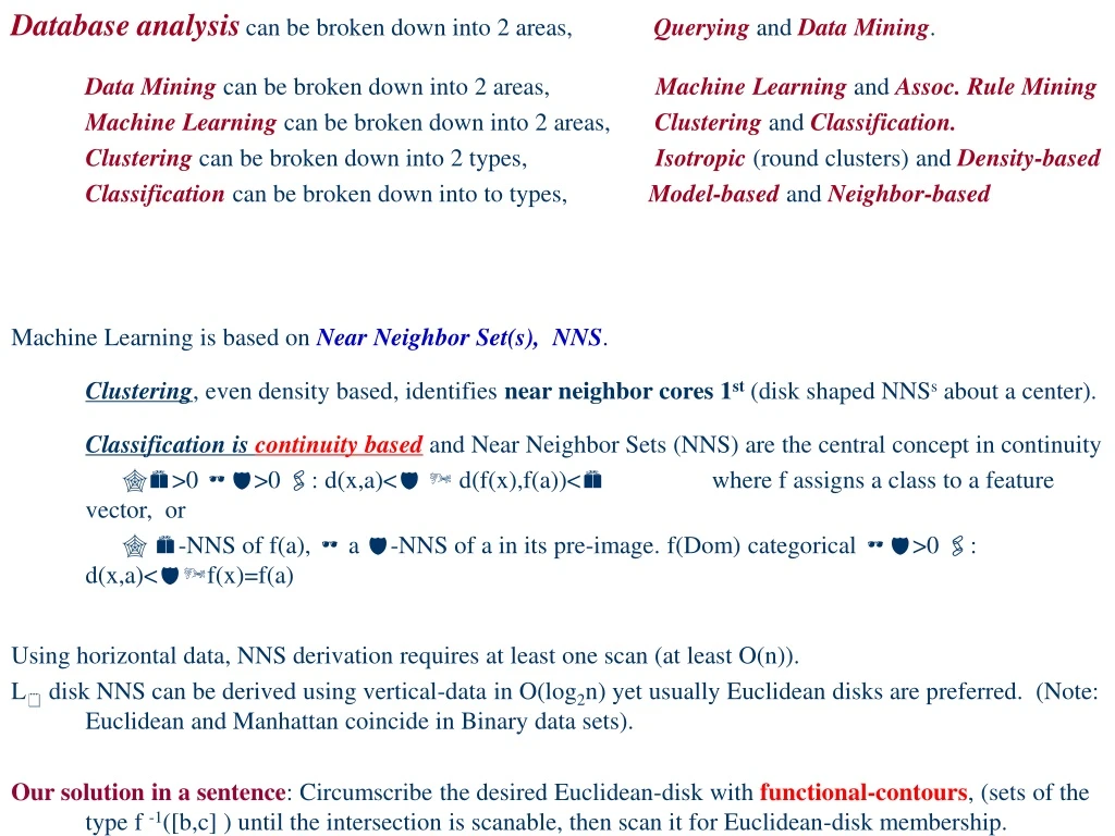
Database analysiscan be broken down into 2 areas, Querying and Data Mining. Data Mining can be broken down into 2 areas, Machine Learning and Assoc. Rule Mining Machine Learning can be broken down into 2 areas, Clustering and Classification. Clustering can be broken down into 2 types, Isotropic (round clusters) and Density-based Classification can be broken down into to types, Model-based and Neighbor-based Machine Learning is based on Near Neighbor Set(s), NNS. Clustering, even density based, identifies near neighbor cores 1st (disk shaped NNSs about a center). Classification is continuity based and Near Neighbor Sets (NNS) are the central concept in continuity >0 >0 : d(x,a)< d(f(x),f(a))< where f assigns a class to a feature vector, or -NNS of f(a), a -NNS of a in its pre-image. f(Dom) categorical >0 : d(x,a)<f(x)=f(a) Using horizontal data, NNS derivation requires at least one scan (at least O(n)). L disk NNS can be derived using vertical-data in O(log2n) yet usually Euclidean disks are preferred. (Note: Euclidean and Manhattan coincide in Binary data sets). Our solution in a sentence: Circumscribe the desired Euclidean-disk with functional-contours, (sets of the type f -1([b,c] ) until the intersection is scanable, then scan it for Euclidean-disk membership. Advantage: intersection can be determined before scanning - create and AND functional contour P-trees.
Contours: f:R(A1..An) Y Equivalently, derived attribute, Af, with domain=Y (equivalence is x.Af = f(x) xR) A1 A2 An : : . . . graph(f) = { ( x, f(x) ) | xR } Y Y R* R f A1 A2 An x1 x2 xn : . . . f(x) A1 A2 An Af x1 x2 xn f(x1..xn) : . . . S x f-contour(S) R Y R f S and SY, the f-contour(S) = f-1(S)Equiv., Af-contour(S) = Select x1..xn From R* Where x.Af=f(x1..xn) If S={a}, we use f-Isobar(a) equiv. Af-Isobar(a) If f is a local density and {Sk} is a partition of Y, {f-1(Sk)} partitions R. (eg, In OPTICS, f=reachability distance, {Sk} is the partition produced by intersections of graph-f wrt to a walk of R and a horizontal line. A Weather map use equiwidth interval partition of S=Reals (barometric pressure or temperature contours). A grid is the intersection partition with respect to the dimension projection functions (next slide). A Class is a contour under f:RC, the class map. An L -disk about a is the intersection of the -dimension_projection contours containing a.
GRIDs 2.lo grid1.hi grid Want square cells or a square pattern? 11 10 01 00 11 10 01 00 000 001 010 011 100 101 110 111 000 001 010 011 100 101 110 111 f:RY, partition S={Sk} of Y, {f-1(Sk)}=S,f-grid of R (grid cells=contours) If Y=Reals, the j.lo f-grid is produced by agglomerating over the j lo bits of Y, fixed (b-j) hi bit pattern. The j lo bits walk [isobars of] cells. Theb-j hi bits identify cells. (lo=extension / hi=intention) Let b-1,...,0 be the b bit positions of Y. The j.lo f-grid is the partition of R generated by f and S = {Sb-1,...,b-j | Sb-1,...,b-j = [(b-1)(b-2)...(b-j)0..0, (b-1)(b-2)...(b-j)1..1)} partition of Y=Reals. If F={fh}, the j.lo F-grid is the intersection partition of the j.lo fh-grids (intersection of partitions). The canonicalj.lo grid is the j.lo -grid; ={d:RR[Ad] | d = dth coordinate projection} j-hi gridding is similar ( the b-j lo bits walk cell contents / j hi bits identify cells). If the horizontal and vertical dimensions have bitwidths 3 and 2 respectively:
j.lo and j.hi gridding continued The horizontal_bitwidth = vertical_bitwidth = b iff j.lo grid = (b-j).hi grid e.g., for hb=vb=b=3 and j=2: 2.lo grid1.hi grid 111 110 101 100 111 110 101 100 011 010 001 000 011 010 001 000 000 001 010 011 100 101 110 111 000 001 010 011 100 101 110 111
r1 r1 a A distance, d, generates a similarity many ways, e.g., s(x,y)=1/(1+d(x,y)): (or if the relationship various by location, s(x,y)=(x,y)/(1+d(x,y)) s r2 1 r2 For C = {a} d s(x,y)=e-d(x,y)2 : s 1 d 0 : d(x,y)> s(x,y)= e-d(x,y)2/std-e-2/std: d(x,y) (vote weighting IS a similarity assignment, so the similarity-to-distance graph IS a vote weighting for classification) s C 1-e-2/std d SOME Useful NearNeighborSets (NNS) Given a similarity s:RRReals and a CR (i.e., s(x,y)=s(y,x); s(x,x)s(x,y) x,yR) Ordinal disks, skins and rings: A disk(C,k) C : |disk(C,k)C'|=k and s(x,C)s(y,C) xdisk(C,k), ydisk(C,k) A skin(C,k)= disk(C,k)-C (skin comes from s k immediate neighbors and is a kNNS of C.) A ring(C,k)= skin(C,k)-skin(C,k-1) closeddisk(C,k)alldisk(C,k); closedskin(C,k)allskin(C,k) Cardinal disk, skins and rings: The disk(C,r) {xR | s(x,C)r} also = functional contour, f-1([r, ), where f(x)=sC(x)=s(x,C) The skin(C,r) disk(C,r) - C The ring(C,r2,r1) disk(C,r2)-disk(C,r1) skin(C,r2)-skin(C,r1) also = functional contour, sC-1(r1,r2] Note: closeddisk and closedskin(C,k) are redundant, since closeddisk(C,k) = disk(C,s(C,y)) where y is any kth NN of C L skins: skin(a,k) = {x | d, xd is one of the k-NNs of ad} - a local normalization?
f:R(A1..An)Y SY The (uncompressed) Predicate-tree0Pf, S is : 0Pf,S(x)=1(true) iff f(x)S 0Pf,S is called a P-tree for short and is just the existential R*-bit mapof SR*.Af The Compressed P-tree,sPf,S is the compression of 0Pf,S with equi-width leaf size, s, as follows 1. Choose a walk of R (converts 0Pf,S from bit map to bit vector) 2. Equi-width partition 0Pf,S with segment size, s (s=leafsize, the last segment can be short) 3. Eliminate and mask to 0, all pure-zero segments (call mask, NotPure0 Mask or EM) 4. Eliminate and mask to 1, all pure-one segments (call mask, Pure1 Mask or UM) (EM=existential aggregation UM=universal aggregation) Compressing each leaf of sPf,S with leafsize=s2 gives: s1,s2Pf,SRecursivly, s1, s2, s3Pf,S s1, s2, s3, s4Pf,S ... (builds an EM and a UM tree) BASIC P-trees If AiReal or Binaryand fi,j(x) jth bit of xi ; {(*)Pfi,j ,{1} (*)Pi,j}j=b..0 are basic (*)P-trees of Ai, *= s1..sk If AiCategorical and fi,a(x)=1 if xi=a, else 0; {(*)Pfi,a,{1}(*)Pi,a}aR[Ai] are basic (*)P-trees of Ai Notes: The UM masks (e.g., of 2k,...,20Pi,j, with k=roof(log2|R| ), form a (binary) tree. Whenever the EM bit is 1, that entire subtree can be eliminated (since it represents a pure0 segment), then a 0-node at level-k (lowest level = level-0) with no sub-tree indicates a 2k-run of zeros. In this construction, the UM tree is redundant. We call these EM trees the basic binary P-trees. The next slide shows a top-down (easy to understand) construction of and the following slide is a (much more efficient) bottom up construction of the same. We have suppressed the leafsize prefix.
A data table, R(A1..An), containing horizontal structures (records) is Vertical basic binary Predicate-tree (P-tree): vertically partition table; compress each vertical bit slice into a basic binary P-tree as follows R( A1 A2 A3 A4) R[A1] R[A2] R[A3] R[A4] 010 111 110 001 011 111 110 000 010 110 101 001 010 111 101 111 101 010 001 100 010 010 001 101 111 000 001 100 111 000 001 100 010 111 110 001 011 111 110 000 010 110 101 001 010 111 101 111 101 010 001 100 010 010 001 101 111 000 001 100 111 000 001 100 Horizontal structures (records) Scanned vertically R11 R12 R13 R21 R22 R23 R31 R32 R33 R41 R42 R43 0 1 0 1 1 1 1 1 0 0 0 1 0 1 1 1 1 1 1 1 0 0 0 0 0 1 0 1 1 0 1 0 1 0 0 1 0 1 0 1 1 1 1 0 1 1 1 1 1 0 1 0 1 0 0 0 1 1 0 0 0 1 0 0 1 0 0 0 1 1 0 1 1 1 1 0 0 0 0 0 1 1 0 0 1 1 1 0 0 0 0 0 1 1 0 0 0 1 0 1 0 0 0 0 1 0 01 0 1 0 0 1 01 1. Whole file is not pure1 0 2. 1st half is not pure1 0 0 0 0 0 1 01 P11 P12 P13 P21 P22 P23 P31 P32 P33 P41 P42P43 3. 2nd half is not pure1 0 0 0 0 0 1 0 0 10 01 0 0 0 1 0 0 0 0 0 0 0 1 01 10 0 0 0 0 1 10 0 0 0 0 1 10 0 0 0 0 1 0 0 0 0 0 0 0 0 0 0 0 0 0 1 1 0 1 0 0 0 0 1 0 1 4. 1st half of 2nd half not 0 0 0 1 0 1 01 5. 2nd half of 2nd half is 1 0 1 0 6. 1st half of 1st of 2nd is 1 Eg, Count number of occurences of 111 000 001 1000 23-level P11^P12^P13^P’21^P’22^P’23^P’31^P’32^P33^P41^P’42^P’43 =0 0 22-level=2 01 21-level 7. 2nd half of 1st of 2nd not 0 processed vertically (vertical scans) then process using multi-operand logical ANDs. R11 0 0 0 0 1 0 1 1 The basic binary P-tree, P1,1, for R11 is built top-down by record truth of predicate pure1 recursively on halves, until purity. But it is pure (pure0) so this branch ends
R11 0 0 0 0 1 0 1 1 Top-down construction of basic binary P-trees is good for understanding, but bottom-up is more efficient. 0 0 0 0 0 1 0 0 0 0 0 1 1 1 Bottom-up construction of P11 is done using in-order tree traversal and the collapsing of pure siblings, as follow: P11 R11 R12 R13 R21 R22 R23 R31 R32 R33 R41 R42 R43 0 1 0 1 1 1 1 1 0 0 0 1 0 1 1 1 1 1 1 1 0 0 0 0 0 1 0 1 1 0 1 0 1 0 0 1 0 1 0 1 1 1 1 0 1 1 1 1 1 0 1 0 1 0 0 0 1 1 0 0 0 1 0 0 1 0 0 0 1 1 0 1 1 1 1 0 0 0 0 0 1 1 0 0 1 1 1 0 0 0 0 0 1 1 0 0 0
Processing Efficiencies? (prefixed leaf-sizes have been removed) R[A1] R[A2] R[A3] R[A4] 010 111 110 001 011 111 110 000 010 110 101 001 010 111 101 111 101 010 001 100 010 010 001 101 111 000 001 100 111 000 001 100 010 111 110 001 011 111 110 000 010 110 101 001 010 111 101 111 101 010 001 100 010 010 001 101 111 000 001 100 111 000 001 100 = R11 R12 R13 R21 R22 R23 R31 R32 R33 R41 R42 R43 0 1 0 1 1 1 1 1 0 0 0 1 0 1 1 1 1 1 1 1 0 0 0 0 0 1 0 1 1 0 1 0 1 0 0 1 0 1 0 1 1 1 1 0 1 1 1 1 1 0 1 0 1 0 0 0 1 1 0 0 0 1 0 0 1 0 0 0 1 1 0 1 1 1 1 0 0 0 0 0 1 1 0 0 1 1 1 0 0 0 0 0 1 1 0 0 0 0 0 1 0 01 0 1 0 1 0 0 1 0 0 1 01 This 0 makes entire left branch 0 7 0 1 4 These 0s make this node 0 P11 P12 P13 P21 P22 P23 P31 P32 P33 P41 P42 P43 These 1s and these 0s make this 1 0 0 0 0 1 01 0 0 0 0 1 0 0 10 01 0 0 0 1 0 0 0 0 0 0 0 1 01 10 0 0 0 0 1 10 To count occurrences of 7,0,1,4 use pure111000001100: 0 P11^P12^P13^P’21^P’22^P’23^P’31^P’32^P33^P41^P’42^P’43 = 0 0 01 0 1 0 ^ ^ ^ ^ ^ ^ ^ ^ ^ 0 0 1 0 1 0 0 1 0 1 01 ^ 0 1 0 R(A1 A2 A3 A4) 2 7 6 1 6 7 6 0 2 7 5 1 2 7 5 7 5 2 1 4 2 2 1 5 7 0 1 4 7 0 1 4 21-level has the only 1-bit so the 1-count = 1*21 = 2
2xRd=1..nad(k2kxdk) + |R||a|2 = xRd=1..n(k2kxdk)2 - 2xRd=1..nad(k2kxdk) + |R||a|2 = xd(i2ixdi)(j2jxdj) - |R||a|2 = xdi,j 2i+jxdixdj- 2 x,d,k2k adxdk + |R|dadad |R||a|2 = x,d,i,j 2i+j xdixdj- = x,d,i,j 2i+j xdixdj- 2|R| dadd + 2 dadx,k2kxdk + TV(a) = i,j,d 2i+j |Pdi^dj| - k2k+1 dad |Pdk| + |R||a|2 dadad ) = x,d,i,j 2i+j xdixdj+ |R|( -2dadd + A useful functional: TV(a) =xR(x-a)o(x-a) If we use d for a index variable over the dimensions, = xRd=1..n(xd2 - 2adxd + ad2) i,j,k bit slices indexes Note that the first term does not depend upon a. Thus, the derived attribute, TV-TV() (eliminate 1st term) is much simpler to compute and has identical contours (just lowers the graph by TV() ). We also find it useful to post-compose a log to reduce the number of bit slices. The resulting functional is called the High-Dimension-ready Total Variation or HDTV(a).
- 2ddad = |R|( dad2 + dd2) g(a) HDTV(a) = ln( f(a) )= ln|R| + ln|a-|2 g(a)=HDTV(x) g(c) g(b) x1 a b c -contour (radius about a) x2 dadad ) TV(a) = x,d,i,j 2i+j xdixdj + |R| ( -2dadd + From equation 7, f(a)=TV(a)-TV() d(adad- dd) ) = |R| ( -2d(add-dd) + = |R| |a-|2 so f()=0 The length of g(a) depends only on the length of a-, so isobars are hyper-circles centered at The graph of g is a log-shaped hyper-funnel: For an -contour ring (radius about a) go inward and outward along a- by to the points; inner point, b=+(1-/|a-|)(a-) and outer point, c=-(1+/|a-|)(a-). Then take g(b) and g(c) as lower and upper endpoints of a vertical interval. Then we use EIN formulas on that interval to get a mask P-tree for the -contour (which is a well-pruned superset of the -neighborhood of a)
use circumscribing Ad-contour (Note: Ad is not a derived attribute at all, but just Ad, so we already have its basic P-trees). If the HDTV circumscribing contour of a is still too populous, (Use voting function, G(x) = Gauss(|x-a|)-Gauss(), where Gauss(r) is (1/(std*2)e-(r-mean)2/2var (std, mean, var are wrt set distances from a of voters i.e., {r=|x-a|: x a voter} ) a -contour (radius about a) • As pre-processing, calculate basic P-trees for the HDTV derived attribute • (or another hypercircular contour derived attribute). • To classify a • 1. Calculate b and c (Depend on a, ) • 2. Form mask P-tree for training pts with HDTV-values[HDTV(b),HDTV(c)] • 3. User that P-tree to prune out the candidate NNS. • If the count of candidates is small, proceed to scan and assign class votes using Gaussian vote function, else prune further using a dimension projections). HDTV(x) HDTV(c) We can also note that HDTV can be further simplified (retaining same contours) using h(a)=|a-|. Since we create the derived attribute by scanning the training set, why not just use this very simple function? Others leap to mind, e.g., hb(a)=|a-b| HDTV(b) x1 contour of dimension projection f(a)=a1 b c x2
HDTV h(a)=|a-| TV-TV() hb(a)=|a-b| TV(x15)-TV() 1 1 2 2 3 3 4 4 5 5 Y X b TV TV(x15) TV()=TV(x33) 1 1 2 2 3 3 4 4 5 5 Y X Graphs of functionals with hyper-circular contours
COS(a) o a ad ad = (1/|a|)d=1..n(xxd) = |R|/|a|d=1..n d = ( |R|/|a| ) ad = |R|/|a|d=1..n((xxd)/|R|) COS(a) a COSb(a)? b a Angular Variation functionals: e.g., AV(a) ( 1/|a| ) xR xoa d is an index over the dimensions, = (1/|a|)xRd=1..nxdad = (1/|a|)d(xxdad) factor out ad COS(a) AV(a)/(|||R|) = oa/(|||a|) = cos(a) COS (and AV) has hyper-conic isobars center on COS and AV have -contour(a) = the space between two hyper-cones center on which just circumscribes the Euclidean -hyperdisk at a. Intersection (in pink)with HDTV -contour. Graphs of functionals with hyper-conic contours: E.g., COSb(a) for any vector, b
Given a training set, R(A1..An,C) the class functional for class attribute value, cC, is functional, f:RC given by f(x)=x.C. The class isobar for class attribute value, cC, f-1(c), is then just the class itself. Since the class functional is one of the dimension projection functionals, it is not a new derived attribute functional (basic P-trees already exist.)
A principle: A job is not done until the Mathematics is completed. The Mathematics of a research job includes 1. Proving claims (theorems, performance evaluation, simulation, etc.), 2. simplification (everything is simple once fully understood), 3. generalization (to the widest possible application scope), and 4. insight (what are the main issues and underlying mega-truths (with full drill down)). Therefore, we need to ask the following questions at this point: Should we use the vector of medians (the only good choice of middle point in mulidimensional space, since the point closest to the mean definition is influenced by skewness, like the mean). We will denote the vector of medians as h(a)=|a-| is an important functional (better than h(a)=|a-|?) If we compute the median of an even number of values as the count-weighted average of the middle two values, then in binary columns, and coincide. (so if µ and are far apart, that tells us there is high skew in the data (and the coordinates where they differ are the columns where the skew is found).
Additional Mathematics to enjoy: What about the vector of standard deviations, ? (computable with P-trees!) Do we have an improvement of BIRCH here? - generating similar comprehensive statistical measures, but much faster and more focused?) We can do the same for any rank statistic (or order statistic), e.g., vector of 1st or 3rd quartiles, Q1 or Q3 ; the vector of kth rank values (kth ordinal values). If we preprocessed to get the basic P-trees of , and each mixed quartile vector (e.g., in 2-D add 5 new derived attributes; , Q1,1, Q1,2, Q2,1, Q2,2; where Qi,j is the ith quartile of the jth column), what does this tell us (e.g., what can we conclude about the location of core clusters? Maybe all we need is the basic P-trees of the column quartiles, Q1..Qn ?) L ordinal disks: disk(C,k) = {x | xd is one of the k-Nearest Neighbors of ad d}. skin(C,k), closed skin(C,k) and ring(C,k) are defined as above. Are they easy P-tree computations? Do they offer advantages? When? What? Why? E.g., do they automatically normalize for us?
Dataset • KDDCUP-99 Dataset (Network Intrusion Dataset) • 4.8 millions records, 32 numerical attributes • 6 classes, each contains >10,000 records • Class distribution: • Testing set: 120 records, 20 per class • 4 synthetic datasets (randomly generated): • 10,000 records (SS-I) • 100,000 records (SS-II) • 1,000,000 records (SS-III) • 2,000,000 records (SS-IV)
Speed and Scalability Speed (Scalability) Comparison (k=5, hs=25) Running Time Against Varying Cardinality 100 Machine: Intel Pentium 4 CPU 2.6 GHz, 3.8GB RAM, running Red Hat Linux Note: these evaluations were done when we were still sorting the derived TV attribute and before we used Gaussian vote weighting. Therefore both speed and accuracy of SMART-TV have improved markedly! SMART-TV 90 PKNN KNN 80 70 60 50 Time in Seconds 40 30 20 10 0 1000 2000 3000 4891 Training Set Cardinality (x1000)
Dataset (Cont.) • OPTICS dataset • 8,000 points, 8 classes (CL-1, CL-2,…,CL-8) • 2 numerical attributes • Training set: 7,920 points • Testing set: 80 points, 10 per class
Dataset (Cont.) • IRIS dataset • 150 samples • 3 classes (iris-setosa, iris-versicolor, and iris-virginica) • 4 numerical attributes • Training set: 120 samples • Testing set: 30 samples, 10 per class
Overall Accuracy Overall Classification Accuracy Comparison
If candidate lies Euclidean distance > from a, vote weight = 0, else, we define Gaussian drop-off function, g(x)= Gauss(r=|x-a|)=1/(std*2 ) * e -(r-mean)2/2var where std, mean, var refer to the set of distances from a of non-zero voters (i.e., the set of r=|x-a| numbers), but use the Modified Gaussian, MG(x) = g(x) - e-2 so the vote weight function drops smoothly to 0 (right at the boundary of the -disk about a and then stays zero outside it). More Mathematics to enjoy: As you probably know, Taufik used a heap process to get the k nearest neighbors of unclassified samples (requiring one scan through the well-pruned nearest neighbor candidate set). This means that Taufik did not use the closed kNN set, so accuracy will be the same as horizontal kNN (single scan, non-closed) Actually, accuracy varies slightly depending on the kth NN picked from the ties). Taufik is planning to leave the thesis that way and explain why he did it that way (over-fairness) ;-) A great learning experience with respect to using DataMIME and a great opportunity for thesis exists here - namely showing that when one uses closed kNN in SMART-TV, not only do we get a tremendously scalable algorithm, but also a much more accurate result (even slightly faster since no heaping to do). A project: Re-run Taufik's performance measurements (just for SMART-TV) using a final scan of the pruned candidate Nearest Neighbor Set. Let all candidates vote using a Gaussian vote drop-off function as:
More Mathematics to enjoy: Meegeum has claimed the study of how much the above improves accuracy in various settings (and how various parameterization of g(x) (ala statistics) affect it)? More enjoyment!: If there is a example data set where accuracy goes down when using the Gaussian and closed NNS, that proves the data set is noise at that point? (i.e., no continuity relationship between features and classes at a). This leads to an interesting theory regarding the continuity of a training set. Everyone assume the training set is what you work with and you assume continuity! In fact, Cancer studies forge ahead with classification even when p>>n, that is there are just too few feature tuples for continuity to even makes good sense! So now we have a method of identifying those regions of the training space where there is a discontinuity in the feature-to-class relationship, FC. That will be valuable (e.g., in Bioinformatics). Has this been studied? (I think, everyone just goes ahead and classifies based on continuity and lives with the result!
More enjoyment (continued): I claim, when the class label is real, then with a properly chosen Gaussian vote-weight function (chosen by domain experts) and with a good method of testing the classifier, if SMART-TV miss-classifies a test point, then it is not a miss-classification at all, but there is a discontinuity in FC there (between feature and class)! In other words, that proves the training set is wrong there and should not be used. I am claiming (do you back me up, Dr. Abidin?) SMART-TV, properly tuned, DEFINES CORRECT! It will be fun to see how far we can go with this point of view. Be warned - it will cause quite a stir! Thoughts: 1. Choose a vote drop-off Gaussian carefully (with domain knowledge in play) and designates it as "right". What could be more right? - if you agree that classification has to be based on FC continuity. 2. Analyze (very carefully) SMART-TV vote histograms for 1 < 2 < ... < h If all are inconclusive then the Feature-to-Class function (FC) is discontinuous at a and classification SHOULD NOT BE ATTEMPTED USING THAT TRAINING SET! (This may get us into Krigging). If the histograms get more and more conclusive as the radius increases, then possibly one would want to rely on the outer ring votes, but one should also report that there is class noise at a! 3. We can get into tuning the Modified Gaussian, MG, by region. Determine the subregion where MC gives conclusive histograms. Then for each inconclusive training point, examine modifications (other parameters or even other dropoff functions) until you find one that is conclusive. Determine the full region where that one is conclusive ...
More enjoyment (continued): CAUTION! Many important Class Label Attributes (CLAs) are real (e.g., level of ill intent in homeland security data mining, level of ill intent in Network Intrusion analysis, probability of cancer in a cancer tissue microarray dataset), but many important Class Label Attributes are categorical (e.g., bioinformatic anotation, Phenotype prediction, etc.). When the Class label is categorical, the distance on the CLA becomes the characteristic distance function (distance=0 iff the 2 categories are different). Continuity at a becomes: >0 :d(x,a)< f(x)=f(a). Possibly boundary determination of the training set classes is most important in case? Is that why SVM works so well in those situations? Still, For there to be continuity at a, it must be the case that some NNS of a maps to f(a). However, if the (CLA) is real: Has anyone every seen analysis of "what is the best definition of correct" done (do statistician do this?). Maybe we need a good statistician to take a look, but let's pursue it anyway so we know what we can claim. Step 1: re-run Taufik's SMART-TV with the Modified Gaussian, MG(x), and closed kNN. We should also take several standard UCI ML classification datasets, randomize classes in some particular isotropic neighborhood (so that we know where there is definitely an FC discontinuity) Then show (using matlab?) that SVM fails to detect that discontinuity (i.e., SVM gives a definitive class to it without the ability to detect the fact that it doesn't deserve one? or do the Lagrange multipliers do that for them?) and then show that we can detect that situation. Does any other author do this? Other fun ideas?
Classifying with multi-relational (heterogeneous) training data 0 0 0 1 0 01 0 1 0 1 0 0 1 0 0 1 01 0 0 0 0 1 01 P11 P12 P13 P21 P22 P23 P31 P32 P33 P41 P42 P43 0 0 0 0 1 0 0 10 01 0 0 0 1 0 0 0 0 0 0 0 1 01 10 0 0 0 0 1 10 0 1 0 0 0 1 0 1 0 0 1 0 1 01 0 1 0 Classify on a foreign key table (S) when some of the features need to come from the primary key table (R)? R(A0 A1 A2) S(B0 B1 B2 B3) 010 111 110 001 011 111 110 000 010 110 101 001 010 111 101 111 101 010 001 100 010 010 001 101 111 000 001 100 111 000 001 100 001 11 0 011 10 1 100 01 1 101 01 0 110 11 0 111 00 0 S11 S12 S13 S21 S22 S23 S31 S32 S33 S41 S42 S43 To data mine this PK multi-relation, (R.A0 is ordered ascending primary key and S.B2 is the foreign key), scan S building (basic P-trees for) the derived attributes Bn+1..Bn+m (here B4,B5) from A1..Am using the bottom up approach (next slide)? Note: Once the derived basic P-trees are built, what if a tuple is added to S? If it has a new B2-value then a new tuples must have been added to R also (with that value in A0). Then all basic P-trees must be extended (including the derived). 0 1 0 1 1 1 1 1 0 0 0 1 0 1 1 1 1 1 1 1 0 0 0 0 0 1 0 1 1 0 1 0 1 0 0 1 0 1 0 1 1 1 1 0 1 1 1 1 1 0 1 0 1 0 0 0 1 1 0 0 0 1 0 0 1 0 0 0 1 1 0 1 1 1 1 0 0 0 0 0 1 1 0 0 1 1 1 0 0 0 0 0 1 1 0 0
R(B2 A1 A2) S(B0 B1 B2 B3) 0 0 1 1 0 1 0 1 1 0 0 1 0 1 0 1 1 0 0 0 0 1 1 1 P01 P02 P03 P11 P12 P13 P21 P22 P23 P31 P32 P33 P4,1 P4,2 P5 0 1 0 0 0 1 0 01 0 1 0 1 0 0 1 0 0 1 01 0 0 0 0 1 01 0 0 0 0 1 0 0 10 01 0 0 0 1 0 0 0 1 1 0 0 0 0 0 0 0 1 01 10 0 0 0 0 1 10 0 1 0 0 0 1 0 1 0 0 1 0 1 01 0 1 0 010 111 110 001 011 111 110 000 010 110 101 001 010 111 101 111 101 010 001 100 010 010 001 101 111 000 001 100 111 000 001 100 001 11 0 011 10 1 100 01 1 101 01 0 110 11 0 111 00 0 S.B4,1 S.B4,2 S.B5 0 1 0 The cost is the same as an indexed nested loop join (reasonable to assume there is a primary index on R). When an insert is made to R, nothing has to change. When an insert is made to S, the P-tree structure is expanded and filled using the values in that insert plus the R-attribute values of the new S.B2 value (This is one index lookup. The S.B2 value must exists in R.A0 by referential integrity). Finally, if we are using, e.g. 4Pi,j P-trees instead of the (4,2,1)Pi,j P-trees shown here, it's the same: The basic P-tree fanout is /\ , the left leaf is filled by the first 4 values, the right leaf is filled with the last 4.
If we are using, e.g. 4Pi,j P-trees instead of the (4,2,1)Pi,j P-trees shown here, it's the same: The basic P-tree fanout is /\ , the left leaf is filled by the first 4 values, the right leaf is filled with the last 4. S.B4,1 S.B4,2 S.B5 0 0 1 S.B4,1 S.B4,2 S.B5 1,1 = EM-S.B4,1 1,1 = EM-S.B4,2 0,0 = EM-S.B5 0,1 = UM-S.B4,1 1,1 = UM-S.B4,2 0,0 = UM-S.B5 1 1 0 0 R(B2 A1 A2) S(B0 B1 B2 B3) 010 111 110 001 011 111 110 000 010 110 101 001 010 111 101 111 101 010 001 100 010 010 001 101 111 000 001 100 111 000 001 100 001 11 0 011 10 1 100 01 1 101 01 0 110 11 0 111 00 0 1 1 1 1 1 1 1 1 1 1 1 1 0 0 0 0 0 0 0 0 1 1 0 0 or
The GO is a data structure which needs to be mined together with various valuable bioinformatic data sets. Biologists waste time searching for all available information about each small area of research. This is hampered further by variations in terminology in common usage at any given time, and that inhibit effective searching by computers as well as people. E.g., In a search for new targets for antibiotics, you want all gene products involved in bacterial protein synthesis, that have significantly different sequence or structure from those in humans. If one DB says these molecules are involved in 'translation' and another uses 'protein synthesis', it is difficult for you - and even harder for a computer - to find functionally equivalent terms. GO is an effort to address the need for consistent descriptions of gene products in different DBs. The project began in 1988 as a collaboration between three model organism databases: FlyBase (Drosophila), Saccharomyces Genome Database (SGD) Mouse Genome Database (MGD). Since then, the GO Consortium has grown to include several of the world's major repositories for plant, animal and microbial genomes. See the GO web page for a full list of member orgs. VertiGO (Vertical Gene Ontology)
The GO is a DAG which needs to be mined in conjunction with the Gene Table (one tuple for each gene with feature attributes). The DAG links are IS-A or PART-OF links. (Description follows from the GO website). If we take the simplified view that the GO assigns annotations of types ( Biological Process (BP); Molecular Function (MF); Cellular Component (CC)) to genes, with qualifiers ( "contributes to", "co-localizes with", "not" ) and evidence codes:IDA=InferredfromDirectAssay; IGI=InferredfromGeneticInteraction, IMP=InferredfromMutantPhenotype; IPI=InferredfromPhysicalInteraction, TAS=TraceableAuthorStatement; IEP=InferredfromExpressionPattern, RCA=InferredfromReviewedComputationalAnalysis, IC=InferredbyCurator IEA=InferredbyElectronicAnnotation ISS=InferredfromSequence/StructuralSimilarity, NAS=NontraceableAuthorStatement, ND=NoBiologicalDataAvailable, NR=NotRecorded Solution-1: For each annotation (term or GOID) have a 2-bit type code column GOIDType BP=11 MF=10 CC=00 and a 2-bit qualifier code column GOIDQualifier with contributesto=11, co-localizeswith=10 and not=00 and a 4-bit evidence code column GOIDEvidence: e,g,: IDA=1111, IGI-1110, IMP=1101, IPI=1100, TAS=1011, IEP=1010, ISS=1001, RCA=1000, IC=0111, IEA=0110, NAS=0100, ND=0010, NR=0001 (putting DAG structure in schema catalog). (Increases width by 8-bits * #GOIDs to losslessly incorporate the GO info). Solution-2: BP, MF and CC DAGs are disjoint (share no GOIDs? true?), an alternative solution is: Use a 4-bit evidencecode/qualifier column, GOIDECQ: For evidence codes: IDA=1111 IGI-1110 IMP=1101 IPI=1100 TAS=1011 IEP=1010 ISS=1001 RCA=1000 IC=0111 IEA=0110 NAS=0101 ND=0100 NR=0011. Qualifiers: 0010=contributesto 0001=colocalizeswith 0000=not (width increases 4-bits*#GOID lossless GO). Solution-3: bitmap all 13 evidencecodes and all 3 qualifiers (adds 16 bit map per GO term). Keep in mind that genes are assumed to be inherited up the DAGs but are only listed at the lowest level to which they apply. This will keep the bitmaps sparse. If a GO term has no attached genes, it need not be included (many such?). It will be in the schema with its DAG links, and will be assumed to inherit all downstream genes, but it will not generate 16 bit columns in Gene Table). Is the not qualifier the complement of the term bitmap? Solution-4: bitmap all 19 attributes (type, qualifiers, evidence codes) VertiGO (Vertical Gene Ontology)
GO has3 structured, controlled vocabularies (ontologies) describing gene products (the RNA or protein resulting after transcription) by their species-independent, associated biological processes (BP), cellular components (CC) molecular functions (MF). There are three separate aspects to this effort: The GO consortium 1. writes and maintains the ontologies themselves; 2. makes associations between the ontologies and genes / gene products in the collaborating DBs, 3. develops tools that facilitate the creation, maintainence and use of ontologies. The use of GO terms by several collaborating databases facilitates uniform queries across them. The controlled vocabularies are structured so that you can query them at different levels: e.g., 1. use GO to find all gene products in the mouse genome that are involved in signal transduction, 2. zoom in on all the receptor tyrosine kinases. This structure also allows annotators to assign properties to gene products at different levels, depending on how much is known about a gene product. GO is not a database of gene sequences or a catalog of gene products GO describes how gene products behave in a cellular context.GO is not a way to unify biological databases (i.e. GO is not a 'federated solution'). Sharing vocabulary is a step towards unification, but is not sufficient. Reasons include: Knowledge changes and updates lag behind.
Curators evaluate data differently (e.g., agree to use the word 'kinase', but not to support this by stating how and why we use 'kinase', and consistently to apply it. Only in this way can we hope to compare gene products and determine whether they are related. GO does not attempt to describe every aspect of biology. For example, domain structure, 3D structure, evolution and expression are not described by GO. GO is not a dictated standard, mandating nomenclature across databases. Groups participate because of self-interest, and cooperate to arrive at a consensus. The 3 organizing GO principles: molecular function, biological process, cellular component. A gene product has one or more molecular functions and is used in one or more biological processes; it might be associated with one or more cellular components. E.g., the gene product cytochrome c can be described by the molecular function term oxidoreductase activity, the biological process terms oxidative phosphorylation and induction of cell death, and the cellular component terms mitochondrial matrix, mitochondrial inner membrane. Molecular function (organizing principle of GO) describes e.g., catalytic/binding activities, at molecular level GO molecular function terms represent activities rather than the entities (molecules / complexes) that perform actions, and do not specify where or when, or in what context, the action takes place. Molecular functions correspond to activities that can be performed by individual gene products, but some activities are performed by assembled complexes of gene products. Examples of broad functional terms are catalytic activity, transporter activity, or binding; Examples of narrower functional terms are adenylate cyclase activity or Toll receptor binding. It is easy to confuse a gene product with its molecular function, and for thus many GO molecular functions are appended with the word "activity". The documentation on gene products explains this confusion in more depth.
A Biological Process is series of events accomplished by 1 or more ordered assemblies of molecular fctns. Examples of broad biological process terms: cellular physiological process or signal transduction. Examples of more specific terms are pyrimidine metabolism or alpha-glucoside transport. It can be difficult to distinguish between a biological process and a molecular function, but the general rule is that a process must have more than one distinct steps. A biological process is not equivalent to a pathway. We are specifically not capturing or trying to represent any of the dynamics or dependencies that would be required to describe a pathway. A cellular component is just that, a component of a cell but with the proviso that it is part of some larger object, which may be an anatomical structure (e.g. rough endoplasmic reticulum or nucleus) or a gene product group (e.g. ribosome, proteasome or a protein dimer). What does the Ontology look like? GO terms are organized in structures called directed acyclic graphs (DAGs), which differ from hierarchies in that a child (more specialized term) can have many parent (less specialized term). For example, the biological process term hexose biosynthesis has two parents, hexose metabolism and monosaccharide biosynthesis. This is because biosynthesis is a subtype of metabolism, and a hexose is a type of monosaccharide. When any gene involved in hexose biosynthesis is annotated to this term, it is automatically annotated to both hexose metabolism and monosaccharide biosynthesis, because every GO term must obey the true path rule: if the child term describes the gene product, then all its parent terms must also apply to that gene product.
It is easy to confuse a gene product and its molecular function, because very often these are described in exactly the same words. For example, 'alcohol dehydrogenase' can describe what you can put in an Eppendorf tube (the gene product) or it can describe the function of this stuff. There is, however, a formal difference: a single gene product might have several molecular functions, and many gene products can share a single molecular function, e.g., there are many gene products that have the function 'alcohol dehydrogenase'. Some, but by no means all, of these are encoded by genes with the name alcohol dehydrogenase. A particular gene product might have both the functions 'alcohol dehydrogenase' and 'acetaldehyde dismutase', and perhaps other functions as well. It's important to grasp that, whenever we use terms such as alcohol dehydrogenase activity in GO, we mean the function, not the entity; for this reason, most GO molecular function terms are appended with the word 'activity'. Many gene products associate into entities that function as complexes, or 'gene product groups', which often include small molecules. They range in complexity from the relatively simple (for example, hemoglobin contains the gene products alpha-globin and beta-globin, and the small molecule heme) to complex assemblies of numerous different gene products, e.g., the ribosome. At present, small molecules are not represented in GO. In the future, we might be able to create cross products by linking GO to existing databases of small molecules such as Klotho , LIGAND
How do terms get associated with gene products? Collaborating databases annotate their gene products (or genes) with GO terms, providing references and indicating what kind of evidence is available to support the annotations. More info in GO Annotation Guide. If you browse any of the contributing databases, you'll find that each gene or gene product has a list of associated GO terms. Each database also publishes a table of these associations, and these are freely available from the GO ftp site. You can also browse the ontologies using a range of web-based browsers. A full list of these, and other tools for analyzing gene function using GO, is available on the GO Tools page . In addition, the GO consortium has prepared GO slims, 'slimmed down' versions of the ontologies that allow you to annotate genomes or sets of gene products to gain a high-level view of gene functions. Using GO slims you can, for example, work out what proportion of a genome is involved in signal transduction, biosynthesis or reproduction. See the GO Slim Guide for more information. All GO data is free. Download the ontology data in a number of different formats, including XML and mySQL, from the GO Downloads page (more info on syntax of these formats, GO File Format Guide. If you need lists of the genes or gene products that have been associated with a particular GO term, the Current Annotations table tracks the number of annotations and provides links to gene association files for each of collaborating DBs is available. GO allows us to annotate genes and their products with a limited set of attributes. e.g., GO does not allow us to describe genes in terms of which cells or tissues they're expressed in, which developmental stages they're expressed at, or their involvement in disease. It is not necessary for GO to this since other ontologies are doing it. The GO consortium supports the development of other ontologies and makes its tools for editing and curating ontologies available. A list of freely available ontologies that are relevant to genomics and proteomics and are structured similarly to GO can be found at the Open Biomedical Ontologies website. A larger list, which includes the ontologies listed at OBO and also other controlled vocabularies that do not fulfil the OBO criteria is available at the Ontology Working Group page of the Microarray Gene Expression Data Society (MGED).
Cross-products: The existence of several ontologies will also allow us to create 'cross-products' that maximize the utility of each ontology while avoiding redundancy. For example, by combining the developmental terms in the GO process ontology with a second ontology that describes Drosophila anatomical structures, we could create an ontology of fly development. We could repeat this process for other organisms without having to clutter up GO with large numbers of species-specific terms. Similarly, we could create an ontology of biosynthetic pathways by combining biosynthesis terms in the GO process ontology with a chemical ontology. Mappings to other classification systems: GO is not the only attempt to build structured controlled vocabularies for genome annotation. Nor is it the only such series of catalogs in current use. We have attempted to make translation tables between these catalogs and GO. We caution that these mappings are neither complete nor exact; they are to be used as a guide. One reason for this is absence of definitions from many of the other catalogs and of a complete set of definitions in GO itself. More information on the syntax of these mappings can be found in the GO File Format Guide. Contributing to GO: The GO project is constantly evolving, and we welcome feedback from all users. If you need a new term or definition, or would like to suggest that we reorganize a section of one of the ontologies, please do so through our online request-tracking system, which is hosted by SourceForge.net. What is a GO term? The purpose of GO is to define particular attributes of gene products. A term is simply the text string used to describe an entry in GO, e.g. cell, fibroblast growth factor receptor binding or signal transduction. A node refers to a term and all its children. GO does not contain the following: Gene products: e.g. cytochrome c is not in GO; attributes of it, e.g., oxidoreductase activity, are. Processes, functions or components that are unique to mutants or diseases: e.g. oncogenesis is not a valid GO term because causing cancer is not the normal function of any gene. Attributes of sequence such as intron/exon parameters: these are not attributes of gene products and will be described in a separate sequence ontology (see OBO web site for more information). Protein domains or structural features. Protein-protein interactions.
Conventions when adding a term: These stylistic points should be applied to all aspects of the ontologies. Spelling conventions: Where there are differences in accepted spelling between English and US, use US form, e.g. polymerizing, signaling, rather than polymerising, signalling. A dictionary of 'words' used in GO terms at GODict.DAT Abbreviations: Avoid abbreviations unless they're self-explanatory. Use full element names, not symbols. Use hydrogen for H+. Use copper and zinc rather than Cu and Zn. Use copper(II), copper(III), etc., rather than cuprous, cupric, etc. For biomolecules, spell out the term in full wherever practical: use fibroblast growth factor, not FGF. Greek symbols: Spell out Greek symbols in full: e.g. alpha, beta, gamma. Case: GO terms are all lower case except where demanded by context, e.g. DNA, not dna. Singular/plural: Use singula, except where a term is only used in plural (eg caveolae). Be descriptive: Be reasonably descriptive, even at the risk of verbal redundancy. Remember, DBs that refer to GO terms might list only the finest-level terms associated with a particular gene product. If the parent is aromatic amino acid family biosynthesis, then child should be aromatic amino acid family biosynthesis, anthranilate pathway, not anthranilate pathway. Anatomical qualifiers: Do not use anatomical qualifiers in the cellular process and molecular function ontologies. For example, GO has the molecular function term DNA-directed DNA polymerase activity but neither nuclear DNA polymerase nor mitochondrial DNA polymerase. These terms with anatomical qualifiers are not necessary because annotators can use the cellular component ontology to attribute location to gene products, independently of process or fctn. Synonyms: When several words or phrases that could be used as the term name, one form will be chosen as term name whilst the other possible names are added as synonyms. Despite the name, GO synonyms are not always 'synonymous' in the strictest sense of the word, as they do not always mean exactly the same as the term they are attached to. Instead, a GO synonym may be broader or narrower than the term string; it may be a related phrase; it may be alternative wording, spelling or use a different system of nomenclature; or it may be a true synonym. This flexibility allows GO synonyms to serve as valuable search aids, as well as being useful for apps such as text mining and semantic matching. Having a single, broad relationship between a GO term and its synonyms is adequate for most search purposes, but for other applications such as semantic matching, the inclusion of a more formal relationship set is valuable. Thus, GO records a relationship type for each synonym, stored in OBO format flat file. Synonym types:The synonym relationship types are: term is an exact synonym (ornithine cycle is an exact synonym of urea cycle) terms are related(cytochrome bc1 complex is a related to ubiquinol-cytochrome-c reductase activity) synonym is broader than the term name (cell division is a broad synonym of cytokinesis) synonym is narrower or more precise(pyrimidine-dimer repair by photolyase is a narrow synonym of photoreactive repair) synonym is related to, but not exact, broader or narrower(virulence has synonym type of other related to term pathogenesis)
These types form a loose hierarchy: related [i] exact synonym [i] broad synonym [i] narrow synonym [i] other related synonym The default relationship is related to, as all synonyms are in some way related to the term name, but more specific relationships are assigned where possible. The synonym type other related is used where the relationship between a term and its synonym is NOT exact, narrower or broader. In some cases, broader and narrower synonyms are created in the place of new parent or child terms because some synonym strings may not be valid GO terms but may still be useful for search purposes. This may be because the synonym is the name of a gene product e.g. ubiquitin-protein ligase activity has the narrower synonym E3, as E3 is a specific gene product with ubiquitin-protein ligase activity. Adding synonyms: When you add a synonym using DAG-Edit, choose a type from the pull-down selector (see the DAG-Edit user guide for more information). DAG-Edit will incorporate the synonym type into the OBO format flat file when you save. The default synonym type is the broadest, 'synonym' (equivalent to 'related' above). Number of synonyms for a term is not limited, and the same text string can be used for more than 1 GO term. Add synonyms if you edit a term name but the old name is still a valid synonym; for example, if you change respiration to cellular respiration, keep respiration as a synonym. This helps other users find familiar terms. Add synonyms if the term has (or contains) a commonly used abbreviation. For example, FGF binding could be used as a synonym for fibroblast growth factor binding. Do not add a synonym if the only difference is case (e.g. start vs. START). Synonyms, like term names, are all lower case except where demanded by context (e.g. DNA, not dna). Rules for Synonyms: Acronyms are exactly synonymous with full name (if acronym is not used in any other sense elsewhere) 'Jargon' type phrases are exactly synonymous w full name (if phrase is not used in any other sense elsewhere) proton is exactly synonymous with hydrogen in most senses EXCEPT where hydrogen means H2 (i.e. gas) include implicit information when making decision; take into account which ontology the term is in - e.g. an entry term that ends in 'factor' is not synonymous with a molecular function. ligand is NOT exactly synonymous with binding (ligand is an entity, binding an action) XXX receptor ligand is NOT exactly synonymous with XXX (1 potential ligands so XXX receptor ligand broader than XXX XXX complex is NOT exactly synonymous with XXX (XXX is ambiguous - could describe activity of XXX) porter and transporter are NOT exactly synonymous (transporter is broader) symporter/antiporter and transporter are NOT exactly synonymous (transporter is broader)
General database cross references (general dbxrefs) should be used whenever a GO term has an identical meaning to an object in another database. Some ex. of common general dbxrefs in GO: Ontology DB Sample dbxref Fctn Enzyme Commission EC:3.5.1.6 Transport Protein Database TC:2.A.29.10.1 Biocatalysis/Biodegradation DB UM-BBD_enzymeID:e0310 Biocatalysis/Biodegradation DB UM-BBD_pathwayID:dcb MetaCyc Metabolic Pathway DB MetaCyc:XXXX-RXN Process MetaCyc Metabolic Pathway DB MetaCyc:2ASDEG-PWY Component None The GO.xrf_abbs file is maintained by the BioMOBY project, so to make changes to the file, you need to use their web form. Understanding relationships in GO: GO ontologies are structured as a directed acyclic graph (DAG), which means that a child (more specialized) term can have multiple parents (less specialized terms). This makes GO a powerful system to describe biology, but creates some pitfalls for curators Keeping the following guidelines in mind should help you to avoid these problems. A child term can have one of two different relationships to its parent(s): is_a or part_of. The same term can have different relationships to different parents; for example, the child 'GO term 3' may be an is_a of parent 'GO term 1' and a part_of parent, 'GO term 2': In GO, an is_a relationship means that the term is a subclass of its parent. For example, mitotic cell cycle is_a cell cycle, not confused with an 'instance' which is a specific example. E.g., clogs are a subclass or is_a of shoes, while the shoes I have on my feet now are an instance of shoes. GO, like most ontologies, does not use instances. The is_a relationship is transitive, which means that if 'GO term A' is a subclass of 'GO term B', and 'GO term B' is an subclass of 'GO term C', 'GO term A' is also a subclass of 'GO term C', E.g., Terminal N-glycosylation is a subclass of terminal glycosylation. Terminal glycosylation is a subclass of protein glycosylation. Terminal N-glycosylation is a subclass of protein glycosylation. part_of in GO is more complex. There are 4 basic levels of restriction for a part_of relationship: 1st type has no restrictions - no inferences can be made from the relationship between parent and child other than that parent may have child as a part, and the child may or may not be a part of the parent.
2nd type, 'necessarily is_part', means that wherever the child exists, it is as part of the parent. To give a biological example, replication fork is part_of chromosome, so whenever replication fork occurs, it is as part_of chromosome, but chromosome does not necessarily have part replication fork. 3rd type, 'necessarily has_part', is the exact inverse of type two; wherever the parent exists, it has the child as a part, but the child is not necessarily part of the parent. For example, nucleus always has_part chromosome, but chromosome isn't necessarily part_of nucleus. 4th type, is a combination of both two and three, 'has_part' and 'is_part'. An example of this is nuclear membrane is part_of nucleus. So nucleus always has_part nuclear membrane, and nuclear membrane is always part_of nucleus. The part_of relationship used in GO is usually type two, 'necessarily is_part'. Note that part_of types 1 and 3 are not used in GO, as they would violate the true path rule. Like is_a, part_of is transitive, so that if 'GO term A' is part_of 'GO term B', and 'GO term B' is part_of 'GO term C', 'GO term A' is part_of 'GO term C': E.g., Laminin-1 is part_of basal lamina. Basal lamina is part_of basement membrane. Laminin-1 is part_of basement membrane. The ontology editing tool DAG-Edit, from version 1.411 on, allows you to specify the necessity of relationships. The part_of relationship used in GO, necessarily is_part, would correspond to part_of, [inverse] necessarily true. For more information, see the DAG-Edit user guide. For info on how these relationships are represented in the GO flat files, see the GO File Format Guide. For technical info on the relationships used in GO and OBO, see the OBO relationships ontology. The true path rule states that "the pathway from a child term all the way up to its top-level parent(s) must always be true". One of the implications of this is that the type of part_of relationship used in GO, outlined more fully in the part_of relationship section above, is restricted to those types where a child term must always be part_of its parent. Often, annotating a new gene product reveals relationships in an ontology that break the true path rule, or species specificity becomes a problem. In such cases, the ontology must be restructured by adding more nodes and connecting terms such that any path upwards is true. When a term is added to the ontology, the curator needs to add all of the parents and children of the new term. This becomes clear with an example: consider how chitin metabolism is represented in the process ontology. Chitin metabolism is a part of cuticle synthesis in fly and is also part of cell wall organization in yeast. This was once represented in process ontology as: cuticle synthesis, [i]chitin metabolism, cell wall biosynthesis, [i]chitin metabolism, ---[i]chitin biosynthesis, ---[i]chitin catabolism
Illustration The problem with this organization becomes apparent when one tries to annotate a specific gene product from one species. A fly chitin synthase could be annotated to chitin biosynthesis, and appear in a query for genes annotated to cell wall biosynthesis (and its children), which makes no sense because flies don't have cell walls. This is revised ontology structure which ensures that the true path rule is not broken: chitin metabolism, [i]chitin biosynthesis, [i]chitin catabolism, [i]cuticle chitin metabolism ---[i]cuticle chitin biosynthesis, ---[i]cuticle chitin catabolism [i]cell wall chitin metabolism, ---[i]cell wall chitin biosynthesis, ---[i]cell wall chitin catabolism Illustration The parent chitin metabolism now has the child terms cuticle chitin metabolism and cell wall chitin metabolism, with the appropriate catabolism and synthesis terms beneath them. With this structure, all the daughter terms can be followed up to chitin metabolism, but cuticle chitin metabolism terms do not trace back to cell wall terms, so all the paths are true. In addition, gene products such as chitin synthase can be annotated to nodes of appropriate granularity in both yeast and flies, and queries will yield the expected results. Dependent ontology terms: Some GO terms imply presence of others. Examples from process ontology include: If either X biosynthesis or X catabolism exists, then parent X metabolism must also exist. If regulation of X exists, then the process X must also exist. Potentially any process in the ontology can be regulated. Note: X may refer to a phenotype (for example cell size in regulation of cell size; in these cases, X should not be added to ontology. GO nodes must avoid using species-specific defs. Nevertheless, many functions, processes and components are not common to all life forms. Our current convention is to include any term that can apply to more than one taxonomic class of organism. Within ontologies, are cases where a word/phrase has different meanings for organisms. E.g., embryonic development in insects is very different from embryonic development in mammals. Such terms are distinguished from one another by their definitions and by the sensu designation (sensu means 'in the sense of'), as in the term embryonic development (sensu Insecta). Nodes should be divided into sensu sub-trees where the children are or are likely to be different. Using sensu designation in a term does not exclude that term from being used to annotate species outside that designation. e.g., a 'sensu Drosophila' term might reasonably used to annotate a mosquito gene product. A GO node should never be more species-specific than any of its children. Child nodes can be at the same level of species specificity as the parent node(s), or more specific. When adding more species-specific nodes, curators should make sure that non-species-specific parents exist (or add them if necessary). E.g., take the process of sporulation. This occurs in both bacteria and fungi, but bacterial sporulation is quite a different process to fungal sporulation, so we therefore add two children to sporulation, sporulation (sensu Bacteria) and sporulation (sensu Fungi). If we now want to add a term to represent the assembly of the spore wall in fungi, we cannot just add spore wall assembly as a direct child of sporulation (sensu Fungi) as such a term could conceivably refer to the assembly of spore walls in bacteria. Name child term spore wall assembly (sensu Fungi) to ensure that it is as species-specific as parent term.
References and Evidence Every annotation must be attributed to a source, which may be a literature reference, another database or a computational analysis. The annotation must indicate what kind of evidence is found in the cited source to support the association between the gene product and the GO term. A simple controlled vocabulary is used to record evidence: IMP inferred from mutant phenotype IGI inferred from genetic interaction <db:gene_symbol[allele_symbol]> IPI inferred from physical interaction [w <db:protein_name>] ISS inferred from sequence similarity [with <database:sequence_id>] IDA inferred from direct assay IEP inferred from expression pattern IEA inferred from electronic annotation [with <database:id>] TAS traceable author statement NAS non-traceable author statement ND no biological data available RCA inferred from reviewed computational analysis IC inferred by curator [from <GO:id>] Annotation File Format: Collaborating databases export to GO a tab delimited file, known informally as a "gene association file" of links between database objects and GO terms. Despite jargon, the db object may represent a gene or a gene product (transcript or protein). Columns in file are described below, a table showing columns in order, with examples, is available. The entry in the DB_Object_ID field (see below) of the association file is the identifier for the database object, which may or may not correspond exactly to what is described in a paper. For example, a paper describing a protein may support annotations to the gene encoding the protein (gene ID in DB_Object_ID field) or annotations to a protein object (protein ID in DB_Object_ID field). The entry in the DB_Object_Symbol field should be a symbol that means something to a biologist, wherever possible (gene symbol, for example). It is not an ID or an accession number (the second column, DB_Object_ID, provides the unique identifier), although IDs can be used in DB_Object_Symbol if there is no more biologically meaningful symbol available (e.g., when an unnamed gene is annotated). The object type (gene, transcript, protein, protein_structure, or complex) listed in the DB_Object_Type field MUST match the database entry identified by DB_Object_ID. Note that DB_Object_Type refers to the database entry (i.e. does it represent a gene, protein, etc.); this column does not reflect anything about the GO term or the evidence on which the annotation is based. For example, if your database entry represents a gene, then 'gene' goes in the DB_Object_Type column, even if the annotation is to a component term relevant to the localization of a protein product of the gene. The text entered in the DB_Object_Name and DB_Object_Symbol can refer to the same database entry (recommended), or to a "broader" entity. For example, several alternative transcripts from one gene may be annotated separately, each with a unique transcript DB_Object_ID, but list the same gene symbol in the DB_Object_Symbol column.
DB refers to the database contributing the gene_association file the value must be present in the file of database abbreviations. [Database abbreviations explanation] this field is mandatory, cardinality 1 DB_Object_ID unique identifier in DB for the item being annotated this field is mandatory, cardinality 1 DB_Object_Symbol (unique and valid) symbol to which DB_Object_ID is matched can use ORF name for otherwise unnamed gene or protein if gene products are annotated, can use gene product symbol if available, or many gene product annotation entries can share a gene symbol this field mandatory, card 1 Qualifier flags that modify interpretation of an annotation 1 (or more) of NOT, contributes_to, colocalizes_with field not mandatory; cardinality 0, 1, >1; for cardinality >1 use a pipe to separate entries (e.g. NOT|contributes_to) GOid GO identifier for the term attributed to the DB_Object_ID this field is mandatory, cardinality 1 DB:Reference one or more unique identifiers for a single source cited as an authority for the attribution of the GOid to the DB_Object_ID. This may be a literature reference or a database record. The syntax is DB:accession_number. Note that only one reference can be cited on a single line in the gene_association file. If a reference has identifiers in more than one database, multiple identifiers for that reference can be included on a single line. For example, if the reference is a published paper that has a PubMed ID, we strongly recommend that the PubMed ID be included, as well as an identifier within a model organism database. Note that if the model organism database has an identifier for the reference, that idenitifier should always be included, even if a PubMed ID is also used. this field is mandatory, cardinality 1, >1; for cardinality >1 use a pipe to separate entries (e.g. SGD:8789|PMID:2676709). The flat file format comprises 15 tab-delimited fields. Blue denotes required fields: Evidence: IMP, IGI, IPI, ISS, IDA, IEP, IEA, TAS, NAS, ND, IC, RCA this is mandatory, cardinality 1 With (or) From one of: DB:gene_symbol; DB:gene_symbol[allele_symbol]; DB:gene_id; DB:protein_nam; DB:sequence_id; GO:GO_id. this field is not mandatory (except in the case of IC evidence code), cardinality 0, 1, >1; for cardinality >1 use a pipe to separate entries (e.g. CGSC:pabA|CGSC:pabB) . Note: This field is used to hold an additional identifier for annotations using certain evidence codes (IC, IEA, IGI, IPI, ISS). For example, it can identify another gene product to which the annotated gene product is similar (ISS) or interacts with (IPI). More information on the meaning of 'with/from' column entries is available in the evidence documentation entries for the relevant codes. Cardinality = 0 is not recommended, but is permitted because cases can be found in literature where no database identifier can be found (e.g. physical interaction or sequence similarity to a protein, but no ID provided). Annotations where evidence is IGI, IPI, or ISS and 'with' cardinality = 0 should link to an explanation of why there is no entry in 'with.' Cardinality may be >1 for any of the evidence codes that use 'with'; for IPI and IGI cardinality >1 has a special meaning. For cardinality >1 use a pipe to separate entries (e.g. FB:FBgn1111111|FB:FBgn2222222). Note that a gene ID may be used in the 'with' column for a IPI annotation, or for an ISS annotation based on amino acid sequence or protein structure similarity, if the database does not have identifiers for individual gene products. A gene ID may also be used if the cited reference provides enough information to determine which gene ID should be used, but not enough to establish which protein ID is correct. 'GO:GO_id' is used only when the evidence code is 'IC', and refers to the GO term(s) used as the basis of a curator inference. In these cases the entry in the 'DB:Reference' column will be that used to assign the GO term(s) from which the inference is made. This field is mandatory for evidence code IC. The ID is usually an identifier for an individual entry in a database (such as a sequence ID, gene ID, GO ID, etc.). Identifiers from the Center for Biological Sequence Analysis (CBS), however, represent tools used to find homology or sequence similarity; these identifiers can be used in the 'with' column for ISS annotations. 'with' col may not be used with evidence codes IDA, TAS, NAS, ND
The flat file format comprises 15 tab-delimited fields. Blue denotes required fields: Aspect one of P (biological process), F (molecular function) or C (cellular component) this field is mandatory; cardinality 1 DB_Object_Name name of gene or gene product. not mandatory, cardinality 0, 1 [white space allowed] Synonym Gene_symbol [or other text]. Strongly recommend gene synonyms are included in the gene association file, as this aids the searching of GO. this field is not mandatory, cardinality 0, 1, >1 [white space allowed]; for cardinality >1 use a pipe to separate entries (e.g. YFL039C|ABY1|END7|actin gene) DB_Object_Type what kind of thing is being annotated one of gene, transcript, protein, protein_structure, complex this field is mandatory, cardinality 1 Taxon taxonomic identifier(s). For cardinality 1, the ID of the species encoding the gene product. For cardinality 2, to be used only in conjunction with terms that have the term 'interaction between organisms' as an ancestor. The first taxon id should be that of the organism encoding the gene or gene product, and the taxon id after the pipe should be that of the other organism in the interaction. mandatory, cardinality 1, 2; for cardinality 2 use a pipe to separate entries (e.g. taxon:1|taxon:1000) Date: on which the annotation was made; format is YYYYMMDD this field is mandatory, cardinality 1 Assigned_by The database which made the annotation one of the values in the table of database abbreviations. [Database abbreviations explanation] Used for tracking the source of an individual annotation. Default value is value entered in column 1 (DB). Value will differ from column 1 for any that is made by one database and incorporated into another. this field is mandatory, cardinality 1 Note that several fields contain database cross-reference (dbxrefs) in the format dbname:dbaccession. The fields are: GOid (where dbname is always GO), DB:Reference, With, Taxon (where dbname is always taxon). For GO ids, do not repeat the 'GO:' prefix (i.e. always use GO:0000000, not GO:GO:0000000)
Computational Annotation Methods This section includes descriptions of automated annotation methods used by participating databases (descriptions have been provided by each group listed). EBI | MGI | TIGR EBI GOA Electronic Annotation The large-scale assignment of GO terms to UniProt Knowledgebase entries involves electronic techniques. This strategy exploits existing properties within database entries including keywords and Enzyme Commission (EC) numbers and cross-reference to InterPro (a database of protein motifs) which are manually mapped to GO. SWISS-PROT keyword and InterPro to GO mappings are maintained in-house and shared on the GO home page for local database updates. Electronically combining these mappings with a table of matching Uniprot Knowledgebase entries generates a table of associations. For each GOA association, an evidence code, which summarizes how the association is made is provided. Associations are made electronically are labeled as 'inferred from electronic annotation' (IEA). Evelyn Camon, 2002-09-03 MGI Electronic Annotation Methods Every object in the MGI databases (markers, seqids, references, etc.) has an MGI: accession ID. See details in GO TIGR ISS Annotation (Arabidopsis, T. brucei) For TIGR Arabidopsis or T. brucei annotations using 'Inferred from Sequence Similarity' (ISS) evidence, the reference is usually 'TIGR_Ath1:annotation' for Arabidopsis (author: TIGR Arabidopsis annotation team) and TIGR_Tba1:annotation for T. brucei (author: TIGR Trypanosoma brucei annotation team), which are defined as follows: name: TIGR annotation based upon multiple sources of similarity evidence description: TIGR_Ath1:annotation or TIGR_Tba1:annotation denotes a curator's interpretation of a combination of evidence. Our internal software tools present us with a great deal of evidence based domains, sequence similarities, signal sequences, paralogous proteins, etc. The curator interprets the body of evidence to make a decision about a GO assignment when an external reference is not available. The curator places one or more accessions that informed the decision in the "with" field. What this says is that we have used many sequence similarity hits, etc., to make our decision. However, we choose only 1-3 pieces of information as "with" information, as it is not practical to enter and submit many entries for each annotation. We also have internal calculations of paralogy and new domains we are identifying which have not yet been published, but which help inform our decisions.