GD Advanced Class Notes

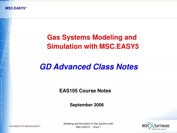
1. Gas Systems Modeling and Simulation withMSC.EASY5 GD Advanced Class Notes EAS105 Course Notes September 2006 Modeling and Simulation of Gas Systems with MSC.EASY5 - Chart 1 E5*V2005*Z*Z*Z*SM*EAS105-NT1

2. Gas Dynamics Class Introduction Goals and Content • Goals • Appreciate MSC.EASY5 as a set of tools to solve hydraulics engineering problems • Use many of MSC.EASY5’s capabilities – and not just the familiar ones • Look for an MSC.EASY5 tool or feature to help with an unusual problem • Work with MSC.EASY5, not around it • What class is not about: • How to design valves and pneumatic systems • MSC.EASY5 mechanics, but some is inevitable • Control analysis/design, but some is inevitable • It will: • Teach you how to use MSC.EASY5 to model pneumatic systems and valves • Review some fundamentals that are usually not well understood • Provide advanced instruction some features of MSC.EASY5 Modeling and Simulation of Gas Systems with MSC.EASY5 - Chart 2

3. Gas Dynamics Class Introduction Outline of Course Content • General Theory of Pneumatic Modeling in MSC.EASY5 • Modeling a Simple Pneumatic Pressure Regulator • Practice basic MSC.EASY5 skills • Obtain Initial Operating Points • Difficulties in Obtaining Steady State • Use Steady State to parameterize models • Modeling a Flow Control Valve • Building Valves from Primitive Pneumatic Components • Building an Electro pneumatic Pressure Regulator • Data Tables and the Matrix Editor • Linear Analysis Modeling and Simulation of Gas Systems with MSC.EASY5 - Chart 3

4. Outline of Course Content • Model a Temperature Control System with Heat Exchangers • Simulation and Numerical Integration • Library Code Development • Sorting and Solving Implicit Loops • Modeling and Development with Discrete Components • Modeling Discontinuities with Switch States • Additional topics as interest and time allows including: • Debugging models • How to define and use your own fluid property set Modeling and Simulation of Gas Systems with MSC.EASY5 - Chart 4

5. Overview of MSC.EASY5 • MSC.EASY5 is an engineering tool for analyzing complex systems • Can be Electrical, Pneumatic, Hydraulic, Mechanical,... • Used for “intermediate” level of detail modeling and analysis • More detailed than discrete event or steady state tools • Less detailed than finite element tools • Models use nonlinear, discontinuous algebraic, differential, and difference equations • Models can be built in different ways • Use MSC.EASY5 general purpose blocks (integrators, saturation, sums,...) • Use MSC.EASY5 libraries for specific application areas • Environmental control • Thermal-hydraulic • Drive train • Vapor cycle • Electric drive • Write your own equations in Fortran components • Build your own application libraries Modeling and Simulation of Gas Systems with MSC.EASY5 - Chart 5

6. Overview of MSC.EASY5 Analysis Options • Types of Analysis: • Steady State • Find the values the plant would settle out to after an initial transient • Simulation – time response • How does the plant respond to a command or a disturbance • Model Linearization • Determine the stability of the system • For control system design • Also for understanding system • Frequency response between any to points in model • Root locus, Stability margins, Eigenvalue Sensitivity, Power Spectral Density • Matrix Algebra Tool • Controls Design • Data Analysis before or after other analyses • Use MSC.EASY5 Plotter to visualize results Modeling and Simulation of Gas Systems with MSC.EASY5 - Chart 6

7. MSC.EASY5 Overview MSC.EASY5 is Several Programs • Programs you interact with • MSC.EASY5 main window • Where you construct your model schematic • Also used for data entry and controlling analyses • Plotter • Visualize the results of the analyses • Icon Editor • Create custom graphic representations for your components • Create component on-line documentation • Matrix Algebra Tool (MAT) • Programs that run in the “background” • Model generator • Translates your schematicdiagram into a Fortran subroutine of model equations called EQMO • Analysis/Simulation program • Where the actual computation occurs • Custom built for each model • Library Maintenance and Model Documentation programs Modeling and Simulation of Gas Systems with MSC.EASY5 - Chart 7

8. MSC.EASY5 Overview Levels of Dynamic System Simulation Fidelity • Physical systems can be simulated at many levels of accuracy. The “correct” level depends on the purpose of the simulation. • 1. Atomic level - Uses equations from quantum mechanics • Purpose: Molecular level effects • Applications: Nuclear physics, quantum chemistry, statisical mechanics • 2. Continuum (or distributed parameter) - Uses partial differential equations • Purpose: Study quantities that vary significantly over the points in a geometric object • Applications: Detailed aerodynamics, impact analysis, component (e.g. valve) analysis • 3.Macroscopic (or lumped parameter) - Uses ordinary differential equations • Purpose: Study quantities that vary in time but can be averaged over spacial components • Applications: Flight controls, hydraulic system analysis, electric power system control • 4.Systems analysis - Uses algebraic equations with time delays • Purpose: Study quantities that effectively change value instantaneously at discrete instances of time • Applications: Scheduling, communications • Each level requires “orders of magnitude more effort than the next highest, • but provides more accurate results. • MSC.EASY5 models dynamic systems at Level 3 (with the occasional 1-Dim Level 2, such as the Method of Characteristics pipe). Modeling and Simulation of Gas Systems with MSC.EASY5 - Chart 8

9. Pneumatics Modeling and Simulation With MSC.EASY5 A Brief Overview of the GD Library Modeling and Simulation of Gas Systems with MSC.EASY5 - Chart 9

10. GD Library Overview • Why is the library called the “Gas Dynamics” Library? • It can be used to model • Pneumatic systems • Environmental control systems • Steam cycles • Gas turbines • Chemically reacting gas systems • Thermal analysis with gases • The scope of the library is much wider than “Pneumatics”, although pneumatic systems modeling is a primary application • It does not model external flows, such as flow around an aircraft wing Modeling and Simulation of Gas Systems with MSC.EASY5 - Chart 10

11. GD Library Overview • Governing equations for fluid flow are represented as ordinary differential equations rather than partial differential equations. • Fluid flow is considered one-dimensional; but this is still a rigorous treatment that includes: • Transient energy effects • Fluid compressibility • No flow or flow reversal possibilities • Transient momentum effects in pipes • Consideration of moisture condensation- important for ECS applications • Gas laws- ideal, Lee-Kestler (built into the library) and user-defined Modeling and Simulation of Gas Systems with MSC.EASY5 - Chart 11

12. Governing Equations • Conservation of Mass • Conservation of Energy • Conservation of Momentum • Flow/Pressure Drop Correlations for Pipes and Orifices • Pipe Friction Factors as a Function of Reynolds Number Modeling and Simulation of Gas Systems with MSC.EASY5 - Chart 12

13. For an ideal gas, this term is zero if Fluid Properties Conservation of Mass or • Density in terms of temperature and (species partial) pressures: Modeling and Simulation of Gas Systems with MSC.EASY5 - Chart 13

14. Conservation of Energy • Energy balance written in terms of enthalpies, temperature and pressure rates: Heat transfer Latent heat Net enthalpy (includes work on fluid by net pressure force) Net kinetic energy • Species mass balances + energy balance form a system of equations that must be solved simultaneously for and. Modeling and Simulation of Gas Systems with MSC.EASY5 - Chart 14

15. Conservation of Momentum, Transient Form • Transient Momentum Balance: shear force convective momentum flux pressure force • Fluid velocity state= v • Friction factor = f (Re,D) • Exit flow = w2 = rvAcs Modeling and Simulation of Gas Systems with MSC.EASY5 - Chart 15

16. Orifice Flow • Orifice flow is based upon isentropic energy balance at steady state. For a single phase: Energy balance Isentropic constraint • Two cases: • Choked:vsis sonic, unknowns arePsandTs • Non-choked:Ps = Pdn, unknowns arevsandTs. • Equations are solved numerically. This approach is applicable to both ideal gases and non-ideal fluids. Flow is then: Modeling and Simulation of Gas Systems with MSC.EASY5 - Chart 16

17. Orifice Conductance • The MSC.EASY5 Gas Dynamics library uses orifice discharge coefficient Cd and orifice area Acs . If the orifice data is in terms of conductance Cv then, if Acs[=] in2 • Only the product Cd Acs can be uniquely determined from Cv. • Therefore, when converting Cv to Cd • Estimate Acs as accurately as you can • Then solve for Cd • Sanity check: 0 < Cd< 1 • Or if an accurate estimate of Acs is impossible • Assume a reasonable value for Cd ( = 0.6-0.8 ) • Solve for Acs Modeling and Simulation of Gas Systems with MSC.EASY5 - Chart 17

18. Switch State Representation of Fluid Flow Regimes Note: Not to scale ZSW = 2 ZSW = 3 ZSW = 3 ZSW = 4 ZSW = 4 W MT -MT Dp 0 choked compressible, not choked choked compressible, not choked Linear Modeling and Simulation of Gas Systems with MSC.EASY5 - Chart 18

19. Body Dynamics Group • The Body Dynamics group contains components to model 1- dimensional mass dynamics of: • Actuator cylinders/diaphragms • Poppets • Spools • Sign convention: a positive force acts in the positive x direction to open the poppet or extend an actuator. • Most Body Dynamics and all Actuator components contain inputs to model coulomb and breakaway friction. • Coulomb friction is a constant force opposing motion. • Breakaway friction does not allow motion until the force on the mass exceeds the breakaway force. • - Breakaway friction must also have a nonzero coulomb friction value. • - Coulomb friction cannot may not exceed breakaway friction. Modeling and Simulation of Gas Systems with MSC.EASY5 - Chart 19

20. Adding Pressure Forces to the Model • There are two convenience components under Forces (CD and CV) that calculate pressure forces. Both determine: • Force = pressure x area • Volume = position x area • Volume rate = velocity x area The NO components represent the actuator extend and retract volumes. They output pressures, which will be converted to force by the CD2. The force calculated by CD2 is, in turn, supplied to PM2. Velocity and position from PM2 are returned to CD2. CD2 supplies volume and volume rate to the NO components. Modeling and Simulation of Gas Systems with MSC.EASY5 - Chart 20

21. Add Pressure Forces to the Model • When connecting the NO or VY components to the CD component, choose the proper port. Remember that the net force is given by: • Net Force = (PP_Volume2*A2 – PP_Volume1*A1)*SGN. Modeling and Simulation of Gas Systems with MSC.EASY5 - Chart 21

22. Add Pressure Forces to the Model You can tell which input connects to which chamber here. Add parameter values to the CD component. Modeling and Simulation of Gas Systems with MSC.EASY5 - Chart 22

23. Strategies for Model Building (or don’t do this at home) • In a training course we: • Cook up problems that are somewhat idealized • Build fairly large models all at once • Provide detailed instructions, parameter values and I.C.s • This optimizes chances for success, efficiently uses class time • This may not work for you outside of a classroom setting • Start small: 1-4 components). Get that working first. • Build incrementally: add 1-4 components at a time. • At each step, carefully consider parameter values and I.C.s, obtain a valid operating point. • Crawl • Walk • Run Modeling and Simulation of Gas Systems with MSC.EASY5 - Chart 23

24. Thermal/Hydraulics Modeling and Simulation With MSC.EASY5 Building a Simple Pressure Regulator Model Modeling and Simulation of Gas Systems with MSC.EASY5 - Chart 24

25. Building a Model • 1.Start MSC.EASY5. • 2. Enter a model name of “PressReg”. • 3. Select the Add button. Modeling and Simulation of Gas Systems with MSC.EASY5 - Chart 25

26. Pressure Regulator • Review the example of a pressure regulator. Outlet orifice diameter: 0.025” Poppet (ball) diameter: 0.188” Seat diameter: 0.135” Regulated pressure: 40 +/- 2 psia Ambient pressure: 8 psia Supply pressure: 150 psia nominal Supply temperature: 580 oF Modeling and Simulation of Gas Systems with MSC.EASY5 - Chart 26

27. Create a Non-venting Pressure Regulator Model 5. Add these components to your schematic pad: Library Group Component gd Miscellaneous GP Fluid Properties gd Boundary Conditions BD Downstream B.C. gd Orifices OR Orifice gd Orifices ORS Orifice gd Orifices ORL Orifice gd Orifice Area PA Poppet Valve Area (vs. position) gd Nodes and Volumes NO Node gd Noces and Volumes VY Variable Volume gd Forces CD Net Pressure Force on Piston gd Forces PF Poppet Valve Aerodynamic Force gd Forces FS Summation of Forces gd Body Dynamics PM Mass Dynamics for Single Mass is -- TI Simulated and accumulated CPU times gp Function Generators AF Analytic Function\Generator Modeling and Simulation of Gas Systems with MSC.EASY5 - Chart 27

28. Component Configurations • 6. Change the “Opening” configuration of component OR from Fixed Diameter to Variable area, external dynamics: • 7. Also change the following configurations: • PA: Concentric with Seat Modeling and Simulation of Gas Systems with MSC.EASY5 - Chart 28

29. Storage Resistive • GD, HC and VC fluid ports: Always make ported connection, otherwise do not connect. • In general, like boundary conditions cannot be connected together. • Components with both inlet and exit storage boundary conditions are labeled. R • Components with both inlet and exit resistive boundary conditions are labeled. S/R • Components with inlet storage and exit resistive boundary conditions are labeled. Component Boundary Conditions S Modeling and Simulation of Gas Systems with MSC.EASY5 - Chart 29

30. Connect Components • Connecting components is a simple process: • Select the “from” component, then select the “to” component • Connect OR to NO • Connect to any available NO inlet port • Examine the connection between OR and NO by double-clicking or middle clicking on the connection line. The ported connection consists of four outputs are connected from OR to NO, and four outputs connected from NO to OR. The connection line is not labeled since more than one output variable is connected. • Connect NO to ORS, to ORL • Connect from any available NO exit port • To select port, Right-H on the To component and select “Create Port Connection” • Connect ORS to VY (use any available VY inlet port) • Connect ORL to BD • 1 ORL exit port, 1 BD inlet port, hence the connection is automatically made. • Finish connecting components • Connect VY (MassDynamics port) to CD (Volume2 port) • Connect CD and PF and to FS • Connect PM to FS • Connect PM to PA • Connect ARE_PA to ARE_OR and ARE_PF • Manually connect S_Out_AF to PP_Inlet1_OR and to PP_P1_PF • Manually connect PP_Inlet1_NO to PP_P2_PF Modeling and Simulation of Gas Systems with MSC.EASY5 - Chart 30

31. Connected Components Rotate and/or flip BD, ORL, ORS, PA & VY icons Modeling and Simulation of Gas Systems with MSC.EASY5 - Chart 31

32. Complex Connections • Connections between the GP components are usually the connection of a single output of the “from” component to a single input of the “to” component. • The real strength of MSC.EASY5 is its ability to use a single connection to represent a physical association between two components of a physical system. • Examples: • Hydraulic fluid flowing from a valve into a heat exchanger • Electric power flowing from a transmission line to a transformer • Mechanical power flowing from a drive shaft to a differential • Modeling these associations requires multi-variable, bi-directional information passing between the component models. • Example: (Hydraulic connection - simplified): Modeling and Simulation of Gas Systems with MSC.EASY5 - Chart 32

33. Port Connections • A component port is a collection of variables (both inputs and outputs) that can be grouped to represent an interface to a physical connection • A port connection between a port on one component to a port on a second component consists of: • A connection of each output variable of either port to the input of the other port with the same quantity name (ignoring the port name) • Ports are named (e.g., “In” “Out” “Shaft”) and are part of the MSC.EASY5 name: Port=In P_In_PD Component=PD Quantity Name=P • Conventional names (W for flow rate, etc.) and ports make automatic connection possible • Also can check for complete connection – i.e. won’t misconnect: • W = flow rate to W = shaft speed because rest of port names don’t match Modeling and Simulation of Gas Systems with MSC.EASY5 - Chart 33

34. } Storage Outlets Resistive } Storage Inlets Resistive Component Pins Aid Connection • Connection points on components are called pins. • Pins can be associated with ports, so that when a connection is made to a component, the connection attaches at the appropriate place on the icon. • MSC.EASY5 pneumatic components use the following convention for pins to help identify what kind of connection can be made. • Connections must be made from Out ports to In ports, and from storage to resistive or resistive to storage. • This translates to: filled pins connect to unfilled pins of the opposite color. Modeling and Simulation of Gas Systems with MSC.EASY5 - Chart 34

35. Gas Properties Components GP and GM • One and only one GP component is required when using any GD components • Defines units, equation of state, gases present in first makeup, ambient temperatures, and pressures • GM components may be used to define additional makeups. Each component that models fluid flow has an input parameter called MUI (make-up index). Component GD/GP always defines MUI=1. Modeling and Simulation of Gas Systems with MSC.EASY5 - Chart 35

36. Gas Properties Components GP and GM • This example of a pneumatically actuated steam valve has 2 makeups: steam (MUI=1) and air (MUI=2). Component GM specifies MUI=2 (air) Component GP specifies MUI=1 (steam) Modeling and Simulation of Gas Systems with MSC.EASY5 - Chart 36

37. Pressure Regulator Source File • Create an executable model: Select Build/Create Executable • Select Build/Display Executable Source File • The source code for this model should look like: • Connections are made by substituting in the name of the output of the ‘from’ component for the name of the input in the code of the ‘to’ component • Notice that the model at this stage has no values for parameters, initial conditions, tables, etc. Modeling and Simulation of Gas Systems with MSC.EASY5 - Chart 37

38. Creating the Executable • MSC.EASY5 • Translates topology - boxes, connections, size of tables - into model generation statements in MSC.EASY5’s language in file model_name.mod • Saves the latest version of your model (model_name.ver.ezmf) if model has changed. • Model file contains no data. • Model file is host-independent - can be processed on any MSC.EASY5 platform. • Places file in your working directory. • Invokes the MSC.EASY5 Model Generator. • MSC.EASY5 Model Generator • Sorts computations in the model into explicit order - every quantity calculated before it is used elsewhere. • MSC.EASY5 can handle some implicit code - see Reference Manual for details. • Generates model description file (model_name.ezmgl). • Generates FORTRAN code representing your model (model_name.f). • Compiles same and binds it with the MSC.EASY5 Analysis Program (model_name.exe). Modeling and Simulation of Gas Systems with MSC.EASY5 - Chart 38

39. Creating the Executable • MSC.EASY5 model of your system • Set of explicit, ordinary differential equations in State Space Form include: • xdot = f(x, time) - derivatives of state variables • y = g(x, time) - formulas for algebraic variables • Implies that calling model with given (x, t) will result in given xdot: • No matter how many times you call it. • No ‘memory’ hidden in model (x = x +1). • State variables are those defined by ordinary differential equations: • They do not change instantaneously. • The states contain all the information needed to stop a simulation and then restart it later. • The numerical integration advances time and recomputes x. • Algebraic variables are just called variables in MSC.EASY5: • They are determined instantaneously by the states. • They don’t need to be saved. Modeling and Simulation of Gas Systems with MSC.EASY5 - Chart 39

40. Define Model Data • 1. Define the model data, both parameter values (Inputs Tab) and initial conditions (States Tab), as given in the following table: Modeling and Simulation of Gas Systems with MSC.EASY5 - Chart 40

41. Define Model Data • 2. Define the model data as given in the following table: Modeling and Simulation of Gas Systems with MSC.EASY5 - Chart 41

42. Define Model Data • 2. Define the model data as given in the following table (continued): Modeling and Simulation of Gas Systems with MSC.EASY5 - Chart 42

43. Calculate Initial Conditions • 3.Select Analysis/Miscellaneous/Initial Condition Calculation. Modeling and Simulation of Gas Systems with MSC.EASY5 - Chart 43

44. Improving the Operating Point • Note on the previous slide that some of the states have large derivatives. • If we were to run a simulation from this operating point (= set of initial conditions for all the states), we would see a sharp transient at the start. • In most cases, this startup transient is non-physical and is only there because we didn’t do a perfect job of guessing initial values for some states in the model. • - For example, even a small error in initializing a pressure state can cause a large initial transient. • Almost all systems have some states for which you don’t know the exact initial value - this value might not even be measurable. • Any analysis we might do at this bad operating point would probably be dominated by this non-physical transient. So, what is the point in doing it? • In large models, this startup transient can be so abrupt as to cause the numerical integration algorithm to FAIL. • Would be nice to have a robust method of removing the errors from an initial operating point. Modeling and Simulation of Gas Systems with MSC.EASY5 - Chart 44

45. Steady State Analysis • Algebraically computes an operating point at which all time derivatives are zero: • This corresponds to the assumption that most plants are normally “at rest.” • Iterative solution based on Newton’s method: • Iteration begins with specified initial conditions. • Default is 100 iterations. • Uses error controls to help manage iteration step sizes. • Computes eigenvalues after last iteration. • Almost always converges: • If initial conditions are not too far off. • If the values make physical sense. • If the values don’t violate assumptions of components (reverse flow not allowed, etc). • If the operating point is not too near a discontinuity, such as a steam/water boundary. Modeling and Simulation of Gas Systems with MSC.EASY5 - Chart 45

46. Graph of f(x) tangent line to graph at (x ,f(x )) k k slope is f(x ) k x Axis crossing point is next guess. x x k+1 k Review of Newton’s Method • Newton’s method is an iterative method for finding a solution to the set of nonlinear equations f(x) = 0. • It requires an initial guess x0 of the solution, which is use to find a better answer x1, which is used to find a better answer x2 that is used to find ...., until some convergence condition of the form abs(f(x)) < eps is satisfied. • Each iteration works as follows: Given xkxk+1 = xk – f(xk)/f'(xk) • Start with xk • Evaluate f(xk ) • Construct point (xk f(xk )) • Construct tangent line to • curve y = f(x) • 5. Find point where tangent • line crosses x-axis. • 6. Call that point xk+1 f'(xk) = δ f(x)|x=xk δx Modeling and Simulation of Gas Systems with MSC.EASY5 - Chart 46

47. Newton’s Method: Multivariate Case • If we are trying to solve the equation f(x) = 0, where f(x)= (f1(x),...,fn(x)) is a vector function of n variables x = (x1,x2,x3,...,xn), then the formula for Newton’s method becomes: • where the -1 exponent denotes matrix inverse and the Jacobian matrix J is the • n x n matrix whose (i,j) element is: • NOTE: The formula above only works if the matrix J is invertable ( i.e. its derivative • is not zero). In the single variable case, this means the tangent line cannot be • horizontal - clearly necessary as seen from the previous graph. • Example of a Singular (non-invertable) system: Consider a model consisting of • a single integrator block whose output does not feed back around to its input. • Then the input is independent of the output so we have Modeling and Simulation of Gas Systems with MSC.EASY5 - Chart 47

48. Not All Systems have a Steady State • Examples: • Rotating machines (shaft velocity never goes to zero, so position never has a zero derivative) • Airplanes (forward velocity better not go to zero) • Open loop systems (integrator output not fed back) • MSC.EASY5 will detect most of these: • Freeze the state (hold the initial condition) • Try the steady state solution • May freeze part of system if initial guess is in dead zone or other flat spot • Looks like an open loop • Try to pick initial guess to bias system out of dead zones Modeling and Simulation of Gas Systems with MSC.EASY5 - Chart 48

49. Strategies for Achieving Steady State • Build models incrementally • Start with 1-4 components • Add a few components at a time • Solve for and save Steady-State operating point at each increment • Obtain stepwise solution by freezing some states • Hydraulics: use “two step method”, freezing temperature states during Step 1 • Hydraulics & pneumatics: freeze position states of pistons, poppets, spools, or other final control elements during Step 1 • Use result of Step 1 as Initial Operating Point of Step 2 • Start with the result of a short simulation. • Make sure all forcing functions have constant values during the simulation • Allows the fastest transients to partially decay • Use the result as the Initial Operating Point of Steady State analysis • Start with trivial steady-state (uniform pressure, zero flow) • Reliable if fluid models allow bi-directional flow • Use steady-state scan Modeling and Simulation of Gas Systems with MSC.EASY5 - Chart 49

50. Finding a Steady State for the Pressure Regulator Model • 1. Select “Analysis/Steady State”. • 2. Toggle the “Save Final Operating Point” to Yes and enter “SteadyState” as the operating point identifier. • 3. Execute the analysis by pressing • 4. Review the results when the results window appears. Modeling and Simulation of Gas Systems with MSC.EASY5 - Chart 50