Download
1 / 25
250 likes | 255 Views
Learn about methods for finding regions in an image and analyzing attributes such as intensity, texture, and shape. Discover how to interpret lines and curves in an image for scene analysis.

E N D
6.4.4 Finding Region • Another method for processing image to find “regions” • Finding regions Finding outlines (c) 2000-2002 SNU CSE Biointelligence Lab
A region of the image • A region is homogeneous. • The difference in intensity values of pixels in the region is no more than some • A polynomial surface of degree k can be fitted to the intensity values of pixels in the region with largest error less than • For no two adjacent regions is it the case that the union of all the pixels in these two regions satisfies the homogeneity property. • Each region corresponds to a world object or a meaningful part of one. (c) 2000-2002 SNU CSE Biointelligence Lab
Split-and-merge method • The algorithm begins with just one candidate region, the whole image. • Until no more splits need be made. • For all candidate regions that do not satisfy the homogeneity property, are each split into four equal-sized candidate regions. • Adjacent candidate regions are merged if their pixels satisfying homogeneity property. (c) 2000-2002 SNU CSE Biointelligence Lab
Regions Found by Split Merge for a Grid-World Scene (from Fig. 6.12) (c) 2000-2002 SNU CSE Biointelligence Lab
“Cleaned Up” the regions found by Split-and-merge method • Eliminating very small regions (some of which are transitions between larger regions). • Straightening bounding lines. • Taking into account the known shapes of objects likely to be in the scene. (c) 2000-2002 SNU CSE Biointelligence Lab
6.4.5 Using Image Attributes Other Than Intensity • Image attributes other than the homogeneity Visual texture • fine-grained variation of the surface reflectivity of the objects • Ex) a field of grass, a section of carpet, foliage in tree, the fur of animals • The reflectivity variations in objects cause similar fine-grained structure in image intensity. (c) 2000-2002 SNU CSE Biointelligence Lab
Methods for analyzing texture • Structural methods • Represent regions in the image by a tessellation of primitive “texels” –small shapes comprising black and white parts • Statistical methods • Based on the idea that image texture is best described by a probability distribution for the intensity values over regions of the image. • Ex) an image of a grassy field in which the blades of grass are oriented vertically a probability distribution that peaks for thin, vertically oriented regions of high intensity, separated by regions of low intensity (c) 2000-2002 SNU CSE Biointelligence Lab
Other attributes • If we had a direct way to measure the range from the camera to objects in the scene, we could produce a “range image” and look for abrupt range differences. • Range image : each pixel value represents the distance from the corresponding point in the scene to the camera. • Motion, color (c) 2000-2002 SNU CSE Biointelligence Lab
6.5 Scene Analysis (1/2) • Scene Analysis • Extracting from the image the needed information about the scene • Requires either additional images (for stereo vision) or general information about the kinds of scenes, since the scene-to-image transformation is many-to-one. • The required knowledge • very general or quite specific • explicit or implicit (c) 2000-2002 SNU CSE Biointelligence Lab
6.5 Scene Analysis (2/2) • Knowledge of surface reflectivity characteristics and shading of intensity in the image give information about the shape of smooth objects in the scene. • Iconic scene analysis • Build a model of the scene or parts of the scene • Feature-based scene analysis • Extracts features of the scene needed by task • Task-oriented or purposive vision (c) 2000-2002 SNU CSE Biointelligence Lab
6.5.1 Interpreting Lines and Curves in the Image • Interpreting the line drawing • Association between scene properties and the components of a line drawing • Trihedral vertex polyhedra • The scene to contain only planar surfaces such that no more than three surfaces intersect in a point Figure 6.15 A Room Scene (c) 2000-2002 SNU CSE Biointelligence Lab
Three kinds of edges in Trihedral vertex polyhedra • There are only three kinds of ways in which two planes can intersect in a scene edge. • Occlude • One kind of edge is formed by two planes, with one of them occluding the other. • labeled in Fig. 6.15 with arrows (). • the arrowhead pointing along the edge such that surface doing the occluding is to the right of the arrow. (c) 2000-2002 SNU CSE Biointelligence Lab
Three kinds of edges in Trihedral vertex polyhedra (2/2) • Blade • Two planes can intersect such that both planes are visible in the scene. • Two surfaces form a convex edge. • Labeled with pluses (+). • Ford • Edge is concave. • Labeled with minus () (c) 2000-2002 SNU CSE Biointelligence Lab
Labels for Lines at Junctions (c) 2000-2002 SNU CSE Biointelligence Lab
Line-labeling scene analysis (1/2) • Labeling all of the junctions in the image as V, W, Y, or T junctions according to the shape of the junctions in the image (c) 2000-2002 SNU CSE Biointelligence Lab
Line-labeling scene analysis (2/2) • Assign +, , or labels to the lines in the image. • An image line that connects two junctions must have a consistent labeling. • If there is no consistent labeling, there must have been some error in converting the image into a line drawing. the scene must no have been one of trihedral polyhedra. • Constraint satisfaction problem (c) 2000-2002 SNU CSE Biointelligence Lab
6.5.2 Model-Based Vision (1/2) • If, we knew that the scene contained a parallelepiped (in Figure 6.15), we could attempt to fit a projection of a parallelepiped to components of an image of this scene. • A generalized cylinders as building blocks for model construction • Each cylinder has 9 parameters. (c) 2000-2002 SNU CSE Biointelligence Lab
Model-Based Vision (2/2) • An example rough scene reconstruction of a human figure • Hierarchical representation • Each cylinder in the model can be articulated into a set of smaller cylinders Figure 6.19 A Scene Model Using Generalized Cylinders (c) 2000-2002 SNU CSE Biointelligence Lab
6.6 Stereo Vision and Depth Information • Depth information can be obtained using stereovision, which based on triangulation calculations using two (or more) images. • Some depth information can be extracted from a single image. • The analysis of texture in the image can indicate that some elements in the scene are closer than are others. • More precise depth information; If we know that a perceived object is on the floor and the camera height above the floor, we can calculate the distance to the object. (c) 2000-2002 SNU CSE Biointelligence Lab
Depth Calculation from a Single Image (c) 2000-2002 SNU CSE Biointelligence Lab
Stereo Vision • Stereo vision uses triangulation. • Two lenses whose centers are separated by a baseline, b. • The image point of a scene point, at distanced, created by these lenses. • The angles of these image points from the lens centers, , . • The optical axes are parallel, the image planes are coplanar, and the scene point is in the same plane as that formed by two parallel optical axes. (c) 2000-2002 SNU CSE Biointelligence Lab
Triangulation in Stereo Vision (c) 2000-2002 SNU CSE Biointelligence Lab
The main complication in stereo vision • In scenes containing more than one point, it must be established which pair of points in the two images correspond to the same scene point. • We must be able to identify a corresponding pixel in the other image. correspondence problem (c) 2000-2002 SNU CSE Biointelligence Lab
Techniques for correspondence problem • Geometric analysis reveals that we need only search along one dimension (epipolarline). • One-dimensional searches can be implemented by cross-correlation of two image intensity profiles along corresponding epipolar lines. • We do not have to find correspondences between individual pairs of image points but can do so between pairs of larger image components, such as lines. (c) 2000-2002 SNU CSE Biointelligence Lab