Download
1 / 19
190 likes | 207 Views
Learn about sorting algorithms like selection, insertion, bubble, merge, quick, stooge, counting, bucket, and radix, as well as how to find the Nth largest/smallest element without sorting.

E N D
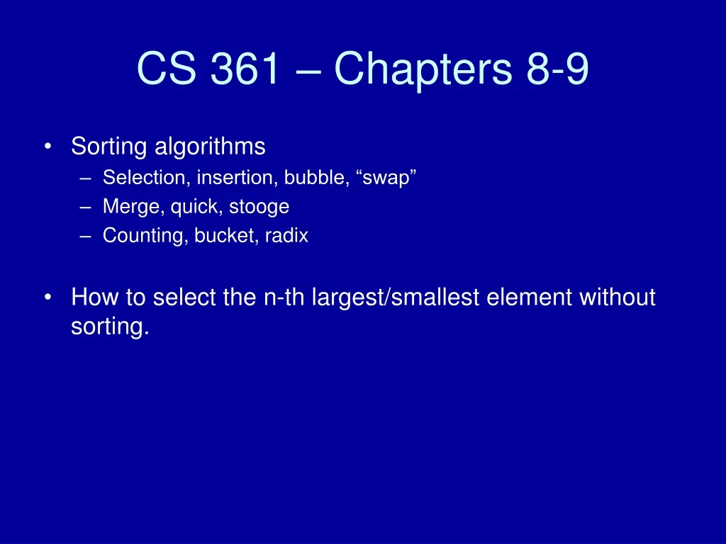
CS 361 – Chapters 8-9 • Sorting algorithms • Selection, insertion, bubble, “swap” • Merge, quick, stooge • Counting, bucket, radix • How to select the n-th largest/smallest element without sorting.
The problem • Arrange items in a sequence so that their keys are in ascending or descending order. • Long history of research. Many new algorithms are tweaks of famous sorting algorithms. • Some methods do better based on how values distributed, size of data, nature of underlying hardware (parallel processing, memory hierarchy), etc. • Some implementations given on the class Web site and also: http://cg.scs.carleton.ca/~morin/misc/sortalg
Some methods • Selection sort: Find the largest value and swap it into first position, find 2nd largest value and put it 2nd, etc. • Bubble sort: Scan the list and see which consecutive values are out of order, and swap them. Multiple passes are required. • Insertion sort: Place the next element in the correct place by shifting other ones over to make room. We maintain a boundary between the sorted and unsorted parts of the list. • Merge sort: Split list in half until just 1-2 elements. Merge adjacent lists by collating them.
Analysis • What is the best case () time for any sorting algorithm? • Selection, bubble, and insertion sort all run in O(n2) time. • Why? • Among the three: which is the best, which is the worst? • Merge sort runs in O(n log2 n) time. • If we imagine the tree of recursive calls, the nested calls go about log2 n deep. At each level, we must do O(1) work at each of the n values. • Later, we will use a more systematic approach to compute the complexity of recursive algorithms.
Quick sort • Like merge sort, it’s a recursive algorithm based on divide and conquer. • Call quickSort initially with parameters (array, 0, n – 1). quickSort(a, p, r): if p < r: q = partition(a, p, r) quickSort(a, p, q) quickSort(a, q+1, r) • What makes quick sort distinctive is its partitioning.
QS partitioning • Given a sub-array spanning indices p..r • Let x = value of first element here, i.e. a[p] • We want to put smaller values on left side and larger values on right side of this array slice. • We return the location of the boundary between the low and high regions.
Counting sort • Designed to run in linear time • Works well when range of values is not large • Find how many values are less than x = a[i]. That will tell you where x belongs in output sorted array. for i = 1 to k: C[i] = 0 for i = 1 to n: // Let C[x] = #elements == x ++ C[A[i]] for i = 2 to k: // Let C[x] = #elements <= x C[i] += C[i – 1] for i = n downto 1: // Put sorted values into B. B[C[A[i]]] = A[i] -- C[A[i]] // try: 3,6,4,1,3,4,1,4
Bucket sort • Assume array’s values are (more or less) evenly distributed over some range. • Create n buckets, each covering 1/n of the range. • Insert each a[i] into the appropriate bucket. • If a bucket winds up with 2+ values, use any method to sort them. • Ex. { 63, 42, 87, 37, 60, 58, 95, 75, 97, 3 } • We can define buckets by tens
Radix sort • Old and simple method. • Sort values based on their ones’ digit. • In other words, write down all numbers ending with 0, followed by all numbers ending with 1, etc. • Continue: Sort by the tens’ digit. Then by the hundreds’ digit, etc. • Can easily be modified to alphabetize words. • Technique also useful for sorting records by several fields.
Stooge sort • Designed to show that divide & conquer does not automatically mean a faster algorithm. • Soon we will learn how to mathematically determine the exact O(g(n)) runtime. stoogeSort(A, i, j): if A[i] > A[j]: swap A[i] and A[j] if i+1 >= j: return k = (j – i + 1) / 3 stoogeSort(A, i, j – k) // how much of A? stoogeSort(A, i + k, j) stoogeSort(A, i, j – k)
Selection • The “selection problem” is: given a sequence of values, return the k-th smallest value, for some k. • If k = 1 or n, problem is simple. • It would be easy to write a O(n log n) algorithm by sorting all values first. But this does unnecessary work. • A randomized method with expected runtime of O(n). • Based on randomized quick sort: choose any value to be the pivot • So it’s called “randomized quick select” • Algorithm takes as input S and k, where 1 k n. (Indices count from 1)
Pseudocode quickSelect(S,k): if n = 1 return S[1] x = random element from S L = [ all elements < x ] E = [ all elements == x ] G = [ all elements > x ] if k <= |L| return quickSelect(L, k) else if k <= |L| + |E| return x else return quickSelect(G, k – |L| - |E|) // e.g. 12th out of 20 = 2nd out of 10
Analysis • To find O(g(n)), we are going to find an upper bound on the “expected” execution time. • Expected, as in expected value – the long term average if you repeated the random experiment many times. • Book has some preliminary notes… • You can add expected values, but not probabilities. • Consider rolling 1 vs. 2 dice. P1(rolling 4) = 1/6 but P2(rolling 8) = 5/36 So the probabilities don’t add! You can only add probability if it’s 2 alternatives of the same experiment, e.g. rolling a 4 or a 5 on one die: 1/6+1/6. • Exp(1 die) = 3.5 Exp(2 dice) = 7 These values can add.
Selection proof • We want to show that the selection algorithm is O(n). • The algorithm is based on partitioning S. • Define a “good” partition = where x is in the middle half of the distribution of values (not in the middle half of locations). • Probability = ½, and sizes of L and of G used for the next recursive call have sizes .75n. • How many recursive calls until we have a “good” partition? Same as asking how many times a coin flips until we get heads: we would expect 2. • Overhead in doing one function invocation. • We need a loop, so this is O(n). Say, bn for some constant b. • T(n) = expected time of algorithm • T(n) T(.75n) + 2bn
Work out recurrence T(n) T(.75n) + 2bn Let’s expand T(.75n) T(.752 n) + 2b(.75n) Substitute: T(n) T(.752 n) + 2b(.75n) + 2bn Expand: T(.752 n) T(.753 n) + 2b(.752 n) Substitute: T(n) T(.753 n) + 2b(.752 n) + 2b(.75n) + 2bn We can keep going and eventually the argument of T on the right side becomes at most 1. (The O(1) base case.) When does that occur? Solve for k: (.75k n) 1 (3/4)k 1/n (4/3)k n k log4/3 n k = ceil(log4/3 n) So, T(n) T(1) + k terms of 2bn multiplied by .75i (for i = 0 to k) (This sum is at most 4.) T(n) O(1) + 2bn (4) = O(n)
Merge sort • We can use the same technique to analyze merge sort. (p. 248). Let’s look at cost of recursive case: T(n) = 2 T(n/2) + cn Expand recursive case: T(n/2) = 2 T(n/4) + c(n/2) Substitute: T(n) = 2 T(n/2) + cn = 2 [ 2 T(n/4) + c(n/2) ] + cn = 4 T(n/4) + 2cn Expand: T(n/4) = 2 T(n/8) + c(n/4) Substitute: T(n) = 4 T(n/4) + cn = 4 [ 2 T(n/8) + c(n/4) ] + 2cn = 8 T(n/8) + 3cn. See a pattern? T(n) = 2k T(n/2k) + kcn At some point, n/2k = 1 n = 2k k = log2 n. T(n) = 2log2 n T(1) + (log2 n) cn = O(n log2 n).
Stooge sort • Yes, even Stooge sort can be analyzed a similar way! T(n) = 3 T((2/3)n) + cn Expand: T((2/3)n) = 3 T((4/9) n) + c((2/3)n) Substitute: T(n) = 3 T((2/3)n) + cn = 3 [ 3 T((4/9) n) + c((2/3)n) ] + cn = 9 T((4/9) n) + 3cn Expand: T((4/9) n) = 3 T((8/27) n) + c((4/9)n) Substitute: T(n) = 9 T((4/9) n) + 3cn = 9 [3 T((8/27) n) + c((4/9)n) ] + 3cn = 27 T((8/27) n) + 7cn Continuing, we observe: T(n) = 3k T((2/3)k n) + (2k – 1)cn
Stooge sort (2) At some point, the recursive argument reaches (or goes below) 1. ((2/3)k n) = 1 (2/3)k = 1/n (3/2)k = n k = log3/2 n So T(n) = 3 log 3/2 n T(1) + (2 log 3/2 n) – 1) cn = O(3 log 3/2 n ) + O(n 2 log 3/2 n) Is this exponential complexity? No – let’s simplify: 3 log 3/2 n = ((3/2) log 3/2 3) log 3/2 n = ((3/2) log 3/2 n) log 3/2 3 = n log 3/2 3 The other term can be simplified similarly and we have n 1 + log 3/2 2 which turns out to be the same order. T(n) = O(n log 3/2 3).