Statistical Quality Control

Statistical Quality Control Chapter 17 To accompanyQuantitative Analysis for Management, Tenth Edition,by Render, Stair, and Hanna Power Point slides created by Jeff Heyl © 2009 Prentice-Hall, Inc.

Define the quality of a product or service • Develop four types of control charts: x, R, p, and c • Understand the basic theoretical underpinnings of statistical quality control, including the central limit theorem • Know whether a process is in control Learning Objectives After completing this chapter, students will be able to:

Chapter Outline 17.1 Introduction 17.2 Defining Quality and TQM 17.3 Statistical Process Control 17.4 Control Charts for Variables 17.5 Control Charts for Attributes

Introduction • Quality is often the major issue in a purchase decision • Poor quality can be expensive for both the producing firm and the customer • Quality management, or quality control (QC), is critical throughout the organization • Quality is important for manufacturing and services • We will be dealing with the most important statistical methodology, statistical process control (SPC)

Defining Quality and TQM • Quality of a product or service is the degree to which the product or service meets specifications • Increasingly, definitions of quality include an added emphasis on meeting the customer’s needs • Total quality management (TQM) refers to a quality emphasis that encompasses the entire organization from supplier to customer • Meeting the customer’s expectations requires an emphasis on TQM if the firm is to complete as a leader in world markets

Defining Quality and TQM • Several definitions of quality • “Quality is the degree to which a specific product conforms to a design or specification.” (Gilmore, 1974) • “Quality is the totality of features and characteristics of a product or service that bears on its ability to satisfy stated or implied needs.” (Johnson and Winchell, 1989) • “Quality is fitness for use.” (Juran, 1974) • “Quality is defined by the customer; customers want products and services that, throughout their lives, meet customers’ needs and expectations at a cost that represents value.” (Ford, 1991) • “Even though quality cannot be defined, you know what it is.” (Pirsig, 1974) Table 17.1

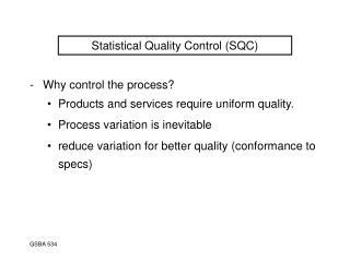
Statistical Process Control • Statistical process control involves establishing and monitoring standards, making measurements, and taking corrective action as a product or service is being produced • Samples of process output are examined • If they fall outside certain specific ranges, the process is stopped and the assignable cause is located and removed • A control chart is a graphical presentation of data over time and shows upper and lower limits of the process we want to control

Upper control limit Target Lower control limit Statistical Process Control Figure 17.1 • Patterns to look for in control charts One plot out above. Investigate for cause. Normal behavior One plot out below. Investigate for cause.

Upper control limit Target Lower control limit Upper control limit Target Lower control limit Statistical Process Control Figure 17.1 • Patterns to look for in control charts Two plots near upper control Investigate for cause. Two plots near lower control. Investigate for cause. Run of 5 above central line. Investigate for cause. Run of 5 below central line. Investigate for cause.

Upper control limit Target Lower control limit Statistical Process Control Figure 17.1 • Patterns to look for in control charts Erratic behavior. Investigate. Trends in either direction 5 plots. Investigate for cause of progressive change.

Statistical Process Control • Building control charts • Control charts are built using averages of small samples • The purpose of control charts is to distinguish between natural variations and variations due to assignable causes

Statistical Process Control • Natural variations • Natural variations affect almost every production process and are to be expected, even when the process is n statistical control • They are random and uncontrollable • When the distribution of this variation is normal it will have two parameters • Mean,  (the measure of central tendency of the average) • Standard deviation,  (the amount by which smaller values differ from the larger ones) • As long as the distribution remains within specified limits it is said to be “in control”

Statistical Process Control • Assignable variations • When a process is not in control, we must detect and eliminate special (assignable) causes of variation • The variations are not random and can be controlled • Control charts help pinpoint where a problem may lie • The objective of a process control system is to provide a statistical signal when assignable causes of variation are present

The x-chart (mean) and R-chart (range) are the control charts used for processes that are measured in continuous units • The x-chart tells us when changes have occurred in the central tendency of the process • The R-chart tells us when there has been a change in the uniformity of the process • Both charts must be used when monitoring variables Control Charts for Variables

The Central Limit Theorem • The central limit theorem is the foundation for x-charts • The central limit theorem says that the distribution of sample means will follow a normal distribution as the sample size grows large • Even with small sample sizes the distribution is nearly normal

We often estimate and with the average of all sample means ( ) The Central Limit Theorem • The central limit theorem says • The mean of the distribution will equal the population mean • The standard deviation of the sampling distribution will equal the population standard deviation divided by the square root of the sample size

Figure 17.2 shows three possible population distributions, each with their own mean () and standard deviation ( ) • If a series of random samples ( and so on) each of size n is drawn from any of these, the resulting distribution of the ‘s will appear as in the bottom graph in the figure • Because this is a normal distribution • 99.7% of the time the sample averages will fall between ±3 if the process has only random variations • 95.5% of the time the sample averages will fall between ±2 if the process has only random variations • If a point falls outside the ±3 control limit, we are 99.7% sure the process has changed The Central Limit Theorem

Normal Beta Uniform  = (mean)  = (mean)  = (mean) x = S.D. x = S.D. x = S.D. 99.7% of all x fall within ±3x 95.5% of all x fall within ±2x | –3x | –2x | –1x | x =  (mean) | +1x | +2x | +3x The Central Limit Theorem • Population and sampling distributions Sampling Distribution of Sample Means (Always Normal) Figure 17.2

where = mean of the sample means z = number of normal standard deviations = standard deviation of the sampling distribution of the sample means = Setting the x-Chart Limits • If we know the standard deviation of the process, we can set the control limits using

A large production lot of boxes of cornflakes is sampled every hour • To set control limits that include 99.7% of the sample, 36 boxes are randomly selected and weighed • The standard deviation is estimated to be 2 ounces and the average mean of all the samples taken is 16 ounces • So and the control limits are Box Filling Example

where = average of the samples A2 = value found in Table 17.2 = mean of the sample means Box Filling Example • If the process standard deviation is not available or difficult to compute (a common situation) the previous equations are impractical • In practice the calculation of the control limits is based on the average range rather than the standard deviation

Factors for Computing Control Chart Limits Table 17.2

 16.01 + (0.577)(0.25)  16.01 + 0.144  16.154  16.01 – (0.577)(0.25)  16.01 – 0.144  15.866 Super Cola Example • Super Cola bottles are labeled “net weight 16 ounces” • The overall process mean is 16.01 ounces and the average range is 0.25 ounces • What are the upper and lower control limits for this process?

We have determined upper and lower control limits for the process average • We are also interested in the dispersion or variability of the process • Averages can remain the same even if variability changes • A control chart for ranges is commonly used to monitor process variability • Limits are set at ±3 for the average range Setting Range Chart Limits

where UCLR = upper control chart limit for the range LCLR = lower control chart limit for the range D4 and D3 = values from Table 17.2 Setting Range Chart Limits • We can set the upper and lower controls using

 (2.114)(53 pounds)  112.042 pounds  (0)(53 pounds)  0 Range Example • A process has an average range of 53 pounds • If the sample size is 5, what are the upper and lower control limits? • From Table 17.2, D4 = 2.114 and D3 = 0

Collect 20 to 25 samples of n = 4 or n = 5 from a stable process and compute the mean and range of each Compute the overall means ( and ), set appropriate control limits, usually at 99.7% level and calculate the preliminary upper and lower control limits. If process not currently stable, use the desired mean, m, instead of to calculate limits. Graph the sample means and ranges on their respective control charts and determine whether they fall outside the acceptable limits Five Steps to Follow in Using x and R-Charts

R-chart Five Steps to Follow in Using x and R-Charts Investigate points or patterns that indicate the process is out of control. Try to assign causes for the variation and then resume the process. Collect additional samples and, if necessary, revalidate the control limits using the new data

Control Charts for Attributes • We need a different type of chart to measure attributes • These attributes are often classified as defective or nondefective • There are two kinds of attribute control charts • Charts that measure the percent defective in a sample are called p-charts • Charts that count the number of defects in a sample are called c-charts

where = mean proportion or fraction defective in the sample z = number of standard deviations = standard deviation of the sampling distribution which is estimated by where n is the size of each sample p-Charts • Attributes that are good or bad typically follow the binomial distribution • If the sample size is large enough a normal distribution can be used to calculate the control limits

ARCO p-Chart Example • Performance of data-entry clerks at ARCO (n = 100)

ARCO p-Chart Example • We want to set the control limits at 99.7% of the random variation present when the process is in control so z = 3 Percentage can’t be negative

Out of Control 0.12 – 0.11 – 0.10 – 0.09 – 0.08 – 0.07 – 0.06 – 0.05 – 0.04 – 0.03 – 0.02 – 0.01 – 0.00 – UCLp = 0.10 Fraction Defective LCLp = 0.00 | 1 | 2 | 3 | 4 | 5 | 6 | 7 | 8 | 9 | 10 | 11 | 12 | 13 | 14 | 15 | 16 | 17 | 18 | 19 | 20 Sample Number ARCO p-Chart Example • p-chart for data entry Figure 17.3

ARCO p-Chart Example • Excel QM’s p-chart program applied to the ARCO data showing input data and formulas Program 17.1A

ARCO p-Chart Example • Output from Excel QM’s p-chart analysis of the ARCO data Program 17.1B

In the previous example we counted the number of defective records entered in the database • But records may contain more than one defect • We use c-charts to control the number of defects per unit of output • c-charts are based on the Poisson distribution which has its variance equal to its mean • The mean is and the standard deviation is equal to • To compute the control limits we use c-Charts

Thus Red Top Cab Company c-Chart Example • The company receives several complaints each day about the behavior of its drivers • Over a nine-day period the owner received 3, 0, 8, 9, 6, 7, 4, 9, 8 calls from irate passengers for a total of 54 complaints • To compute the control limits

Statistical Quality Control