Download
1 / 90
920 likes | 1.12k Views
When advection destroys balance, vertical circulations arise. ppt started from one by James T. Moore Saint Louis University Cooperative Institute for Precipitation Systems. Brian Mapes. COMET-MSC Winter Weather Course 29 Nov. - 10 Dec. 2004. Quasi-Geostrophic Theory.

E N D
When advection destroys balance, vertical circulations arise ppt started from one by James T. Moore Saint Louis University Cooperative Institute for Precipitation Systems Brian Mapes COMET-MSC Winter Weather Course 29 Nov. - 10 Dec. 2004
Quasi-Geostrophic Theory • It provides a framework to understand the evolution of balanced three-dimensional velocity fields. • It reveals how the dual requirements of hydrostatic and geostrophic balance (encapsulated as thermal wind balance) constrain atmospheric motions. • It helps us to understand how the balanced, geostrophic mass and momentum fields interact on the synoptic scale to create vertical circulations which result in sensible weather.
Stable balanced dynamics • Deviations from balance lead to force imbalances that drive ageostrophic and vertical motions which adjust the state back toward balance. • Consider hydrostatic, geostrophic as simplest case of balances. • Houze chapter 11 - use Boussinesq, hydrostatic equation set as we did for gravity waves. • Introduce pseudoheight • Assume wind is mostly geostrophic ug, vg • Note: f-plane approximation means Vg =0
Balance in atmospheric dynamics • The vertical equation of motion: imbalance between the 2 terms on the RHS results in small vertical motions that restore balance - unless the state is gravitationally unstable • The horizontal equation of motion: imbalance between the major terms on the RHS leads to small ageostrophic motions that restore balance - unless the state is inertially unstable • Between lies symmetric instability. Like gravitional instability, it has moist (potential, conditional) cousins. For now, STABLE CASE
Old school: Quasi-Geostrophic Omega Equation (vorticity-oriented form) A B C Term A: three-dimensional Laplacian of omega Term B: vertical variation of the geostrophic advection of the absolute geostrophic vorticity Term C: Laplacian of the geostrophic advection of thickness
Problems with the Traditional Form of Q-G Diagnostic Omega Equation • The two forcing functions are NOT independent of each other • The two forcing functions often oppose one another (e.g., PVA and cold air advection – who wins?) • You need more than one level of information to estimate differential geostrophic vorticity advection • You cannot estimate the Laplacian of the geostrophic thickness advection by eye! • The forcing functions depend upon the reference frame within which they are measured (i.e., the forcing functions are NOT Galilean invariant)
PV view of how maintenance of balance requires vertical motions
warm Thermal wind balance prevails: There is a Z trough (trof) for geostrophic balance, with a cold core beneath it, supporting it hypsometrically (in hydrostatic balance). cyclonic z (Trof) COOL CORE
Unshearedadvection of T, u, v, vort, PV: no problem, whole structure moves warm cyclonic (Trof) COOL CORE
Sheared advection breaks thermal wind balance warm cyclonic z (Trof) COOL CORE
Sheared advection breaks thermal wind balance Coriolis forces COOL CORE Z Trof (hypsometric)
Sheared advection breaks thermal wind balance imbalanced force = acceleration COOL CORE Z Trof (hypsometric)
The PV view of balanced circulation: (Rob Rogers’s fig) Potential temperature and potential vorticity cross sections Long-lived Great Plains MCV Hurricane Andrew after landfall
Q-vector Form of the Q-G Diagnostic Omega Equation Alternate approach developed by Hoskins et al. (1978, Q. J.) – manipulated the equations so forcing is 1 term, not 2:
Q-vector Form of the Q-G Diagnostic Omega Equation Treat Laplacian as a “sign flip” Then, If -2•Q > 0 (convergence of Q)then w < 0 (upward vertical motion) If -2•Q < 0 (divergence of Q)then w > 0 (downward vertical motion) The Q vector points along the ageostrophic wind in the lower branch of the secondary circulation Q vectors point toward the rising motion and are proportional to the strength of the horizontal ageostrophic wind
Advantages of Using Q Vectors • You only need one isobaric level to compute the total forcing (although layers are probably better to use) • Only one forcing term, so no cancellation between terms • Plotting Q vectors indicates where the forcing for vertical motion is located and they are a good approximation for the ageostrophic wind • The forcing function is not dependent on the reference frame (I.e., it is Galilean invariant • Plotting Q vectors and isentropes can indicate regions of Q-G frontogenesis/frontolysis • No term is neglected (as in the Trenberth method which neglects the deformation term)
Interpreting Q Vectors Expanding Q and assuming adiabatic conditions yields the following expression for Q: Setting aside the coefficients,
Interpretation of Qx Geostrophic stretching deformation weakens Geostrophic shearing deformation turns cold vg ug cold warm to warm cold to+t cold warm warm
Interpretation of Qy Geostrophic shearing deformation turns Geostrophic stretching deformation strengthens cold vg ug cold warm to warm cold to+t cold warm warm
An Alternative form of Q in “natural” coordinates Keyser et al. (1992, MWR) derived a form of the Q vector in “natural” coordinates where one component is oriented parallel to isotherms and another component is oriented normal to the isotherms. In this form one component (Qs) has the two shearing deformation terms, expressing rotation of isotherms, that normally show up in Qx and Qy . Meanwhile, the other component (Qn) has the two stretching deformation terms expressing the contraction or expansion of isotherms. We will see that this novel form of the Q vector has distinct advantages, in terms of interpretation.
Defining the Orientation of Qs and Qn with Respect to Qn Q cold -1 Qs +1 +2 n warm s Qs is the component of Q associated with rotating the thermal gradient. Qn is the component of Q associated with changing the magnitude of the thermal gradient. Martin (1999, MWR) Keyser et al. (1992, MWR)
DefiningQn and Interpreting What It Means (cont.) +1 • Couplets of div Qn: • Tend to line up across the isotherms • Show the ageostrophic response to the geostrophically-forced packing/unpacking of the isotherms • Often exhibit narrow banded structures typical of the “frontal” scale • Give an indication of how “active” a front might be +2 Qn vg/y < 0; therefore Qn <0; Qn points from cold to warm air; confluence (diffluence) in wind field implies frontogenesis (frontolysis)
Interpreting Q vectors: Qn Advection by geostrophic stretching deformation acts to change the magnitude of the thermal gradient vector, . But the same geostrophic advection changes the wind shear in the direction OPPOSITE to that needed to restore balance. This is why the forcing for ageostrophic secondary circ is -2x(.Q)! Low level wind: pure geostrophic deformation (noting .Vg = 0), here acting to weaken dT/dx. cold warm Upper level wind: addthermal windtolow levelwind. v component is positive and decreases to north, so advection is acting to increase upper-level v. Thermal wind
Thermal wind Upper wind DefiningQs and Interpreting What It Means (cont.) • Couplets of div Qs: • Tend to line up along the isotherms • Show the ageostrophic response to the geostrophically-forced turning of the isotherms • Tend to be oriented upstream and downstream of troughs • Are associated with the synoptic wave scale of ascent and descent +1 +2 Qs Qs vg/x > 0; therefore Qs > 0. Qs has cold air is to its left, causes cyclonic rotation of the vector . Thermal wind balance thus requires v to increase aloft, but geostrophic advection acts to decrease v aloft.
Estimating Q vectors Sanders and Hoskins (1990, WAF) derived a form of the Q vector which could be used when looking at weather maps to qualitatively estimate its direction and magnitude: Where the x axis is defined to be along the isotherms (with cold air to the left) and y is normal to x and to the left. Thus, Q is large when the temperature gradient is strong and when the geostrophic shear along the isotherms is strong. To estimate the direction of Q just use vector subtraction to compute the derivative of Vg along the isotherms, then rotate the vector by 90° in the clockwise direction. Example:
A B - Col Region B A = Q vectors 90 deg Q A B B A - Jet Entrance Region = 90 deg This is mainly the cross-front, n component Qn Q Holton (1992)
Q vectors in a setting where warm air rises cold Qn vectors warm Direct Thermal Circulation Confluent Flow Holton, 1992
Q vectors in a setting where COLD air rises Jet Exit Region Q Vageo Thermally Indirect Circulation Vageo South North
Idealized pattern of sea-level isobars (solid) and isotherms (dashed) for a train of cyclones and anticyclones. Heavy bold arrows are Q vectors. This is mostly the along-front or s component Qs. Holton (1992)
Semi-geostrophic extension to QG theory • Allow advection of b and v by an ageostrophic horizontal wind uain cross-front (x) direction only(following Houze section 11.2.2). • An elegant trick: define • Using the fact that Dvg/Dt = -fua, the total derivative in X space • becomes analogous to Dg/Dt:
Semi-geostrophic extension to QG theory (cont) • More elegant trickery: • Defining the geostrophic PV (Houze 11.50) • One can get the streamfunction equation (11.60) • Comparing the QG case (11.20) • PV plays the role of a static stability in this system.
Another form (from notes of R. Johnson, CSU) is met (translation: PV must be positive, so that the system is symmetrically stable)
Frontogenesis (definition) (S. Petterssen 1936) • The 2-D scalar frontogenesis function (F ): • F > 0 frontogenesis, F < 0 frontolysis • F: generalization of the quasi-geostrophic version, the Q-vector • Can also include diabatic heating gradients, etc. g Q
Symmetric instabilities, contributing to banded precipitation, often north and east of midlatitude cyclones
Mesoscale Instabilities and Processes Which Can Result in Enhanced Precipitation • Conditional Instability • Convective Instability • Inertial Instability • Potential Symmetric Instability • Conditional Symmetric Instability • Weak Symmetric Stability • Convective-Symmetric Instability • Frontogenesis
Balance in atmospheric dynamics • The vertical equation of motion: imbalance between the 2 terms on the RHS results in small vertical motions that restore balance - unless the state is gravitationally unstable • The horizontal equation of motion: imbalance between the major terms on the RHS leads to small ageostrophic motions that restore balance - unless the state is inertially unstable • Between lies symmetric instability. Like gravitional instability, it has moist (potential, conditional) cousins. For now, STABLE CASE
Instabilities: nomenclatureSchultz et al. MWR 1999 “The intricacies of instabilities”
Conditional Symmetric Instability: Cross section of esand Mg taken normal to the 850-300 mb thickness contours s es-1 es es+ 1 Mg +1 Symm. unstable Note: isentropes of es are sloped more vertical than lines of absolute geostropic momentum, Mg. Mg Vert. stable Horiz. stable Mg -1
Conditional Symmetric Instability in the Presence of Synoptic Scale Lift – Slantwise Ascent and Descent Multiple Bands with Slantwise Ascent
Frontogenesis and varying Symmetric Stability • Emanuel (1985, JAS) has shown that in the presence of weak symmetric stability (simulating condensation) in the rising branch, the ageostrophic circulations in response to frontogenesis are changed. • The upward branch becomes contracted and becomes stronger. The strong updraft is located ahead of the region of maximum geostrophic frontogenetical forcing. • The distance between the front and the updraft is typically on the order of 50-200 km • On the cold side of the frontogenetical forcing stability is greater and and the downward motion is broader and weaker than the updraft.
Frontal secondary circulation - constant stability Emanuel (1985, JAS) Frontal secondary circ - with condensation on ascent
Schematic of Convective-Symmetric Instability Circulation Blanchard, Cotton, and Brown, 1998 (MWR)
Convective-Symmetric Instability Multiple Erect Towers with Slantwise Descent
Sanders and Bosart, 1985: Mesoscale Structure in the Megalopolitan Snowstorm of 11-12 February 1983. J. Atmos. Sci.,42, 1050-1061.