Download
1 / 39
390 likes | 580 Views
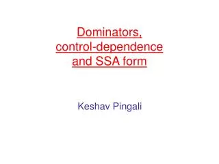
Dominators, control-dependence and SSA form. Organization. Dominator relation of CFGs postdominator relation Dominator tree Computing dominator relation and tree Dataflow algorithm Lengauer and Tarjan algorithm Control-dependence relation SSA form. Control-flow graphs. START.

E N D
Organization • Dominator relation of CFGs • postdominator relation • Dominator tree • Computing dominator relation and tree • Dataflow algorithm • Lengauer and Tarjan algorithm • Control-dependence relation • SSA form
Control-flow graphs START • CFG is a DAG • Unique node START from which all nodes in CFG are reachable • Unique node END reachable from all nodes • Dummy edge to simplify discussion START END • Path in CFG: sequence of nodes, possibly empty, such that successive nodes in sequence are connected in CFG by edge • If x is first node in sequence and y is last node, we will write the path as x * y • If path is non-empty (has at least one edge) we will write x + y a b c d e f g END
Dominators START • In a CFG G, node a is said to dominate node b if every path from START to b contains a. • Dominance relation: relation on nodes • We will write a dom b if a dominates b a b c d e f g END
Example START START A B C D E F G END x x x x x x x x x A START A B C D E F G END x x x x x x x B x x x x x x C x x D E x x F x x G END
Computing dominance relation • Dataflow problem: Domain: powerset of nodes in CFG Dom_out(N) = {N} U Dom_in(N) N Confluence operation: set intersection Find greatest solution Work through example on previous slide to check this. Question: what do you get if you compute least solution?
Properties of dominance • Dominance is • reflexive: a dom a • anti-symmetric: a dom b and b dom a a = b • transitive: a dom b and b dom c a dom c • tree-structured: • a dom c and b dom c a dom b or b dom a • intuitively, this means dominators of a node are themselves ordered by dominance
Example of proof • Let us prove that dominance is transitive. • Given: a dom b and b dom c • Consider any path P: START + c • Since b dom c, P must contain b. • Consider prefix of P = Q: START + b • Q must contain a because a dom b. • Therefore P contains a.
Dominator tree example START START a b a END c c b d e f f e d g g END Check: verify that from dominator tree, you can generate full relation
Computing dominator tree • Inefficient way: • Solve dataflow equations to compute full dominance relation • Build tree top-down • Root is START • For every other node • Remove START from its dominator set • If node is then dominated only by itself, add node as child of START in dominator tree • Keep repeating this process in the obvious way
Building dominator tree directly • Algorithm of Lengauer and Tarjan • Based on depth-first search of graph • O(E*a(E)) where E is number of edges in CFG • Essentially linear time • Linear time algorithm due to Buchsbaum et al • Much more complex and probably not efficient to implement except for very large graphs
Immediate dominators • Parent of node b in tree, if it exists, is called the immediate dominator of b • written as idom(b) • idom not defined for START • Intuitively, all dominators of b other than b itself dominate idom(b) • In our example, idom(c) = a
Useful lemma • Lemma: Given CFG G and edge ab, idom(b) dominates a • Proof: Otherwise, there is a path P: START + a that does not contain idom(b). Concatenating edge ab to path P, we get a path from START to b that does not contain idom(b) which is a contradiction. START a END c b f e d g fb is edge in CFG Idom(b) = a which dominates f
Postdominators • Given a CFG G, node b is said to postdominate node a if every path from a to END contains b. • we write b pdom a to say that b postdominates a • Postdominance is dominance in reverse CFG obtained by reversing direction of all edges and interchanging roles of START and END. • Caveat: a dom b does not necessarily imply b pdom a. • See example: a dom b but b does not pdom a
Obvious properties • Postdominance is a tree-structured relation • Postdominator relation can be built using a backward dataflow analysis. • Postdominator tree can be built using Lengauer and Tarjan algorithm on reverse CFG • Immediate postdominator: ipdom • Lemma: if a b is an edge in CFG G, then ipdom(a) postdominates b.
Control dependence • Intuitive idea: • node w is control-dependent on a node u if node u determines whether w is executed • Example: START e START ….. if e then S1 else S2 …. END S1 S2 m END We would say S1 and S2 are control-dependent on e
Examples (contd.) START e START ….. while e do S1; …. END S1 END We would say node S1 is control-dependent on e. It is also intuitive to say node e is control-dependent on itself: - execution of node e determines whether or not e is executed again.
Example (contd.) • S1 and S3 are control-dependent on f • Are they control-dependent on e? • Decision at e does not fully determine if S1 (or S3 is executed) since there is a later test that determines this • So we will NOT say that S1 and S3 are control-dependent on e • Intuition: control-dependence is about “last” decision point • However, f is control-dependent on e, and S1 and S3 are transitively (iteratively) control-dependent on e START e f S2 S3 S1 n END m
Example (contd.) • Can a node be control-dependent on more than one node? • yes, see example • nested repeat-until loops • n is control-dependent on t1 and t2 (why?) • In general, control-dependence relation can be quadratic in size of program n t1 t2
Formal definition of control dependence • Formalizing these intuitions is quite tricky • Starting around 1980, lots of proposed definitions • Commonly accepted definition due to Ferrane, Ottenstein, Warren (1987) • Uses idea of postdominance • We will use a slightly modified definition due to Bilardi and Pingali which is easier to think about and work with
Control dependence definition • First cut: given a CFG G, a node w is control-dependent on an edge (uv) if • w postdominates v • ……. w does not postdominate u • Intuitively, • first condition: if control flows from u to v it is guaranteed that w will be executed • second condition: but from u we can reach END without encountering w • so there is a decision being made at u that determines whether w is executed
Control dependence definition • Small caveat: what if w = u in previous definition? • See picture: is u control-dependent on edge uv? • Intuition says yes, but definition on previous slides says “u should not postdominate u” and our definition of postdominance is reflexive • Fix: given a CFG G, a node w is control-dependent on an edge (uv) if • w postdominates v • if w is not u, w does not postdominate u u v
Strict postdominance • A node w is said to strictly postdominate a node u if • w != u • w postdominates u • That is, strict postdominance is the irreflexive version of the dominance relation • Control dependence: given a CFG G, a node w is control-dependent on an edge (uv) if • w postdominates v • w does not strictly postdominate u
Example START a b c d e f g a x x x x STARTa fb cd ce ab x x x b x c x x d e f g END
Computing control-dependence relation • Nodes control dependent on edge (uv) are nodes on path up the postdominator tree from v to ipdom(u), excluding ipdom(u) • We will write this as [v,ipdom(u)) • half-open interval in tree END g START f c e d a b a b c d e f g x x x x STARTa fb cd ce ab x x x x x x
Computing control-dependence relation • Compute the postdominator tree • Overlay each edge uv on pdom tree and determine nodes in interval [v,ipdom(u)) • Time and space complexity is O(EV). • Faster solution: in practice, we do not want the full relation, we only make queries • cd(e): what are the nodes control-dependent on an edge e? • conds(w): what are the edges that w is control-dependent on? • cdequiv(w): what nodes have the same control-dependences as node w? • It is possible to implement a simple data structure that takes O(E) time and space to build, and that answers these queries in time proportional to output of query (optimal) (Pingali and Bilardi 1997).
SSA form • Static single assignment form • Intermediate representation of program in which every use of a variable is reached by exactly one definition • Most programs do not satisfy this condition • (eg) see program on next slide: use of Z in node F is reached by definitions in nodes A and C • Requires inserting dummy assignments called F-functions at merge points in the CFG to “merge” multiple definitions • Simple algorithm: insert F-functions for all variables at all merge points in the CFG and rename each real and dummy assignment of a variable uniquely • (eg) see transformed example on next slide
SSA example START START A A Z0:= … Z:= … Z1 := F(Z4,Z0) p1 B B p1 C C …… Z3:= F(Z1,Z3) D Z2:= …. D Z:= …. G p3 p3 G E E Z4:= F(Z2,Z3) p2 p2 print(Z) F print(Z4) F END END
Minimal SSA form • In previous example, dummy assignment Z3 is not really needed since there is no actual assignment to Z in nodes D and G of the original program. • Minimal SSA form • SSA form of program that does not contain such “unnecessary” dummy assignments • See example on next slide • Question: how do we construct minimal SSA form directly?
Dominance frontier • Dominance frontier of node w • Node u is in dominance frontier of node w if w • dominates a CFG predecessor v of u, but • does not strictly dominate u • Dominance frontier = control dependence in reverse graph! A B C D E F G A B C DEFG x x Example from previous slide x x x
Iterated dominance frontier • Irreflexive closure of dominance frontier relation • Related notion: iterated control dependence in reverse graph • Where to place F-functions for a variable Z • Let Assignments = {START} U {nodes with assignments to Z in original CFG} • Find set I = iterated dominance frontier of nodes in Assignments • Place F-functions in nodes of set I • For example • Assignments = {START,A,C} • DF(Assignments) = {E} • DF(DF(Assignments)) = {B} • DF(DF(DF(Assignments))) = {B} • So I = {E,B} • This is where we place F-functions, which is correct
Why is SSA form useful? • For many dataflow problems, SSA form enables sparse dataflow analysis that • yields the same precision as bit-vector CFG-based dataflow analysis • but is asymptotically faster since it permits the exploitation of sparsity • see lecture notes from Sept 6th • SSA has two distinct features • factored def-use chains • renaming • you do not have to perform renaming to get advantage of SSA for many dataflow problems
Computing SSA form • Cytron et al algorithm • compute DF relation (see slides on computing control-dependence relation) • find irreflexive transitive closure of DF relation for set of assignments for each variable • Computing full DF relation • Cytron et al algorithm takes O(|V| +|DF|) time • |DF| can be quadratic in size of CFG • Faster algorithms • O(|V|+|E|) time per variable: see Bilardi and Pingali
Dependences • We have seen control-dependences. • What other kind of dependences are there in programs? • Data dependences: dependences that arise from reads and writes to memory locations • Think of these as constraints on reordering of statements
Data dependences • Flow-dependence (read-after-write): S1S2 • Execution of S2 may follow execution of S1 in program order • S1 may write to a memory location that may be read by S2 • Example: ….. x := 3 …x.. ……. while e do …x… x: = … …… flow-dependence flow-dependence This is called a loop-carried dependence
Anti-dependences • Anti-dependence (write-after-read): S1S2 • Execution of S2 may follow execution of S1 in program order • S1 may read from a memory location that may be (over)written by S2 • Example: x := … ..x…. x:= … anti-dependence
Output-dependence • Output-dependence (write-after-write): S1S2 • Execution of S2 may follow execution of S1 in program order • S1 and S2 may both write to same memory location
Summary of dependences • Dependence • Data-dependence: relation between nodes • Flow- or read-after-write (RAW) • Anti- or write-after-read (WAR) • Output- or write-after-write (WAW) • Control-dependence: relation between nodes and edges