Download
1 / 41
410 likes | 562 Views
GPU-based Visualization Algorithms. Han-Wei Shen Associate Professor Department of Computer Science and Engineering The Ohio State University . Scientific Visualization. A process of converting numerical data into visual images

E N D
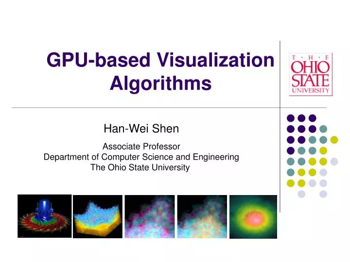
GPU-based Visualization Algorithms Han-Wei Shen Associate Professor Department of Computer Science and Engineering The Ohio State University
Scientific Visualization • A process of converting numerical data into visual images • The images should contain useful information to help the scientist to obtain understanding about his/her data
Applications • Large Scale Time-Dependent Simulations • Richtmyer-Meshkov Turbulent Simulation (LLNL) • 2048x2048x1920 grid per time step (7.7 GB) • Run 27,000 time steps • output size > 2 TB LLNL IBM ASCI system
Applications • Oak Ridge Terascale Supernova Initiative (TSI) • 640x640x640 floats • > 1000 time steps • Total size > 1 TB • NASA’s turbo pump simulation • Multi-zones • Moving meshes • 300+ time steps • Total size > 100GB ORNL TSI data NASA turbo pump
Current Research Projects • Time-Varying Data Visualization • Flow Visualization • View Dependent Algorithms • Parallel Rendering
Time-Varying Data Visualization • Key - Data are huge (~100 TBs) • Research: • Spatio-Temporal Multiresolution Hierarchy • Feature Tracking • High Dimensional Rendering
Flow Visualization • Key – visualize the dynamics • Research • Texture synthesis and animation • Streamline placements
View Dependent Algorithms • Key – Give the user the best view with a minimal effort • Research • Occlusion culling • Automatic view selection
Parallel Rendering • Key – have an optimal utilization of computation resources (CPU and storage) • Research • Large format display • Dynamic Load Balancing
Computer Graphics Technology Has advanced at an amazing speed
The Programmable GPU • GPU = vertex shader (vertex program) + fragment shader (fragment program, pixel program) • Vertex shader replaces per-vertex transform & lighting • Fragment shader replaces texture stages • Fragment testing after the fragment shader • Flexibility to do framebuffer pixel blending Vertex Shader Fragment Shader vertices Transform And Lighting Clipping Primitive Assembly And Rasterization Texture Stages Fragment Testing primitives
GPU-based Wavelet Reconstruction • Wavelets are useful for multiresolution analysis and compression of 3D volumetric datasets. • Previous 3D wavelet solutions are mostly implemented by convolution operators or by software. • Our work reconstructs 3D wavelets using the GPUs.
H0 H1 H2 ... L0 L1 L2 ... Wavelet Theory • Wavelets are defined on basis functions that filter a set of original values (A values) into low-frequency coefficients (L values) and high-frequency coefficients (H values). • L values are also known as averages, and H values as details. A0 A1 A2 A3 A4 A5 ...
2 x(2d x d) 4 x(d x d) H L HH HL LH LL Y transform X transform 2D Wavelet Transform • For two- or three-dimensional data, wavelets are applied successively on each dimension, which creates 4 or 8 coefficient bricks respectively 2d x 2d
HH HL H L LH LL y z Y transform X transform x HHH HHL HLH HLL LHH LHL LLH LLL 3D Wavelet Transform • A volume of (2d)3 voxels will be transformed into 8 of d3 bricks of coefficients Z transform
HH HL H L y LH LL z X reconstruction x Y reconstruction HHH HHL HLH HLL LHH LHL LLH LLL Z reconstruction 3D Wavelet Reconstruction • Reconstruct the original volume of (2d)3 from the 8 d3 bricks of coefficients
3D Wavelet Reconstruction • A straightforward implementation of 3D wavelet reconstructions involves a large number of texture copying • Render-to-texture feature is not available for 3D textures • More efficient algorithm is needed to take advantage of the GPUs
LLL LLL LLL LLL LLL LLL y z x Tileboards • Tileboard: flatten a 3D brick into 2d tiles LLL LLL LLL LLL = LLL LLL LLL
LLL LLL LLL LLL LLL LLL LLL LLL LLL = LLL LLL LLL LLL y z x Tileboards • Tileboard: flatten a 3D brick into 2d tiles • Merge HLL, HLH, HHL, HHH into a RGBA texture HHH HHL HLH HLL LHH LHL LLH LLL
LLL LLL LLL LLL LLL LLL y z x HLL HLH HHH HHL HHL HLL HHH HLH HLH HLL HHH HHL HLH HHH HLL HHL HLL HLH HHL HHH HHL HLL HLH HHH Tileboards • Tileboard: flatten a 3D brick into 2d tiles • Merge HLL, HLH, HHL, HHH into a 2D RGBA texture LLL LLL LLL LLL = LLL LLL LLL HHH HHL HLH HLL LHH LHL LLH LLL
LLL LLL LLL LLL LLL LLL y z x LLL LLH LHH LHL LHL LLL LHH LLH LLH LLL LHH LHL LLH LHH LLL LHL LLL LLH LHL LHH LHL LLL LLH LHH Tileboards • Tileboard: flatten a 3D brick into 2d tiles • Merge LLL, LLH, LHL, LHH into a single 2D RGBA texture LLL LLL LLL LLL = LLL LLL LLL HHH HHL HLH HLL LHH LHL LLH LLL
H- and L-Tileboard • Pack the 8 coefficient bricks into H- and L-Tileboards
Reconstruction • The use of tileboards allows us to retrieve 4 coefficients at a single texture lookup (2 2D RGBA textures) Evaluating wavelet reconstruction formula for each fragment 2d of 2d x 2d tiles In pbuffer H-Tileboard Proxy polygon L-Tileboard
Reconstruction Details • Z reconstruction: combine HHH and LHH, HHL and LHL, HLH and LLH, HLL and LLL HHH HHL HLH HLL LHH LHL LLH LLL Z reconstruction
Reconstruction Details • Z reconstruction: combine HHH and LHH, HHL and LHL, HLH and LLH, HLL and LLL R G B A HHH HHL HLH HLL H Tileboard LHH LHL LLH LLL Z reconstruction L Tileboard
Reconstruction Details • Z reconstruction: combine RGBA from H- and L- Tileboard (z reconstruction – H** and L**) • Harr wavelets: • O RGBA = (H RGBA + L RGBA)/sqrt(2) (even z) • O RGBA = (H RGBA - L RGBA)/sqrt(2)(odd z) +
HH HL LH LL Reconstruction Details • Y reconstruction: combine HH and LH, HL and LL HHH HHL LHL LHH HLH HLL LLH LLL Y reconstruction
Reconstruction Details • Y reconstruction: combine HH and LH, HL and LL • HH + LH = A + G • HL + LL = R + B HH HL LH LL
H L y z x Reconstruction Details • X reconstruction: combine H and L
Reconstruction Details • Z reconstruction • O RGBA = (H RGBA + L RGBA)/sqrt(2) (even z) • O RGBA = (H RGBA - L RGBA)/sqrt(2) (odd z) • Y reconstruction • O H = O A + O G • O L = O R + O B • X reconstruction • O = OH + OL +
Reconstruction Details • Z reconstruction • O RGBA = (H RGBA + L RGBA)/sqrt(2) (even z) • O RGBA = (H RGBA - L RGBA)/sqrt(2) (odd z) • Y reconstruction • O H = O A + O G • O L = O R + O B • X reconstruction • O = OH + OL Single Fragment Pass +
Pseudocode float4 haar( float2 c : TEX0, // Coords in output tileboard space uniform samplerRECT LTileboard, // L-Tileboard uniform samplerRECT HTileboard) : COLOR // H-Tileboard { float3 d = CoordsTile2Dto3D(c); // Coords in 3D brick space float2 e = Coords3DtoTile2D(d / 2); // Coords in L- and H-tileboard space float4 L = texRECT(LTileboard, e); // Fetch (LLL, LLH, LHL, LHH) float4 H = texRECT(HTileboard, e); // Fetch (HLL, HLH, HHL, HHH) float4 RZ = L + H * ChooseSign(d.z); // Reconstruct in Z float2 RY = RZ.rg + RZ.ba * ChooseSign(d.y); // Reconstruct in Y float RX = RY.r + RY.g * ChooseSign(d.x); // Reconstruct in X return Color(RX); // return A value } float ChooseSign(float x) { return 1 – 2 * fmod(x, 2); } // 1 or -1
Reconstructed Tileboard Final image Rendering • The goal is NOT to read out the reconstructed data from the pbuffer • 3D volume rendering is performed using the reconstructed tileboard directly 3D volume slicing and rendering
Results • Both Harr and Daubechies wavelets were implemented • Experiments were done on 3.0 GHz Xeon processor with nVidia Quadro FX 3400 card
CPU v.s. GPU (in seconds) Visible woman data set:480^3 Brick size: 64x64x64
Brick Sizes v.s. Reconstruction Time (in msec) Time includes uploading and reconstruction
Drop coefficient bricks • Coefficients can be dropped to trade quality for speed Reconstruction time for the visible woman data using different numbers of coefficient bricks (in seconds)
Drop coefficient bricks • Dropping bricks affects image quality, which is more severe with Haar than with Daubechies wavelets. Harr Daubechies
Multiresolution Rendering • Multiresolution can be achieved by feeding the reconstructed tileboard to the next resolution level.
Conclusions • We have devised an algorithm that can successfully utilize GPUs to reconstruct 3D wavelet coefficients. • We have also embedded our implementation in multiresolution data hierarchies.
Ongoing Efforts • Encode and reconstruct of time-varying data • Parallel algorithms for visualizing large scale data