1 / 0

Theories applied to Chemistry

1. Theories applied to Chemistry. Applies to all chemical systems. Quantum Mechanics (Planck, Einstein, Schrödinger - Ĥ Y =E Y). Wave-particle duality allows mathematical wave function solutions to predict chemical properties of systems. Incorporates Heisenberg Uncertainty Principle.

dessa
Download Presentation

Theories applied to Chemistry

An Image/Link below is provided (as is) to download presentation Download Policy: Content on the Website is provided to you AS IS for your information and personal use and may not be sold / licensed / shared on other websites without getting consent from its author. Content is provided to you AS IS for your information and personal use only. Download presentation by click this link. While downloading, if for some reason you are not able to download a presentation, the publisher may have deleted the file from their server. During download, if you can't get a presentation, the file might be deleted by the publisher.

E N D

Presentation Transcript


  1. 1 Theories applied to Chemistry Applies to all chemical systems. Quantum Mechanics (Planck, Einstein, Schrödinger - ĤY=EY). Wave-particle duality allows mathematical wave function solutions to predict chemical properties of systems. Incorporates Heisenberg Uncertainty Principle. The behavior of individual particles are not certain, but represented as outcome probabilities. Statistical treatments make measurements on large systems essentially certain. Although QM is the primary theory explaining the behavior of subatomic particles, atoms, and molecules it gives way to CM for much of chemistry due to its more complex mathematical foundations.
  2. Theories applied to Chemistry Classical Mechanics (Newton’s Laws of Motion?) Applies only to larger (atoms /molecules), slower (relative to c) particles. Although CM leads to a number of inconsistencies in chemical behavior it is still used for chemical topics where it provides accurate predictions with more conceptually accessible explanations. CM topics in chemistry include much of kinetics and thermodynamics.
  3. Theories applied to Chemistry Classical Mechanics (Newton - e.g. F = ma) There are two distinct approaches to studying classical systems in chemistry …. Macroscopic Look at behavior of system as whole (P vs. V at cst T) Summarize behavior as a set of laws (Boyle’s Law etc.) Develop equations predicting the behavior of systems. (P1V1 = P2V2) Microscopic (Classical) Develop a physical model explaining molecular behavior. Apply Laws of motion to individual particles. Extrapolate to collection of particles (statistical mechanics). Derive equations predicting the behavior of systems(CM).
  4. y z x Kinetic Molecular Theory (KMT) see handout Assume: 1. gas particles have mass but no volume 2. particles in constant, random motion 3. no attractive/repulsive forces 4. conservation of energy at every collision
  5. vy vz vx y z x Pressure of Ideal Gas P = F/A & PA = F = ma = m(dvx/dt) = dpx/dt dpx= 2mvx dpx= ? dt= 2x/vx dt= ? PA = 2mvx/(2x/vx) = mvx2/x PAx = PV = mvx2 For N molecules ― PV = Nm<vx2> = nM<vx2> v2 = vx2 + vy2 + vz2 & <v2> = 3<vx2 > & …. <vx2> = <v2>/3 PV = nM<v2>/3 = nRT <v2> = 3nRT/nM = 3RT/M <v2>1/2 = vrms = (3RT/M)1/2
  6. vy vz vx y z x Pressure of Ideal Gas P = F/A & F = ma = dpx/dt = nRT PV = Nm<v2>/3 = nM<v2>/3 Derive expression for <v2>1/2 = vrms Derive expression for KE (Etr) = ½nM<v2> in terms of T.
  7. <v2>1/2 = vrms = (3RT/M)1/2 use KE (etr) = ½mv2from Newton’s 2nd Law …to derive an expression for KE (Etr) = in terms of T. Etr = ½Nm<v2> = ½nM<v2> for N particles = nRT PV = Nm<v2>/3 = nM<v2>/3 x 3/2 Etr = ½nM<v2> = 3nRT/2 Or …. Etr,m = 3RT/2 (per mole) etr = 3kT/2 (per molecule)since R = NAk or nR = Nk rms-speed is a function of both T and M …… Kinetic energy is only a function of T In the KMT all gases have an ‘equal’ impact on P at a fixed T, because the greater force of larger particles is offset by their slower speed
  8. 2 The Barometric Formula This derivation is not in your text (see handout). However, it illustrates one practical application of statistical mechanics … The approximate atmospheric content as a function of altitude … This model also serves as an example of the Boltzman Distribution Law, a law derived using statistical mechanics, that illustrates how particles distribute themselves over an energy gradient. The Boltzman Distribution law is fundamental both to CM and QM. In the latter it is required to explain the characteristics of spectroscopy arising from the population distribution of quantum states. We will apply the Boltzman Distribution law as a shortcut to avoid a more exact but tedious derivation of the speed distribution function.
  9. Barometric Formula & Boltzmann Distribution z = altitude dz = thickness of atmosphere layer A = Surface area of layer What is Fup and Fdown? Fup = PA Fdown = g • dm + (P + dP)A dm = mass of gas between z & dz dP = Pressure difference between z & z + dz.
  10. Barometric Formula Let Fup = Fdown PA = (dm)g + (P + dP)A dm/M PV = nRT & n = ? dm = MPV/RT PA = MPVg/RT + PA + dP • A & dP = -MPVg/ART Since V/A = dz …. dP/P = -Mgdz/RT integrate PºP dP/P = -Mg/RT 0z dz ln (P/P) = -Mgz/RT &... P = P exp(-Mgz/RT)
  11. Boltzmann Distribution Law by analogy to Barometric Formula P/P = exp(-Mgz/RT) P/P ~ N/No& DE (J/mol) = -Mgz(kg•m2•s-2/mol) J = kg•m2•s-2 N/No= exp(-DE/RT) or.... N/No= exp(-De/kT) The Boltzmann Distribution Law gives the relative occupation for any two energy levels. e.gheight in gravitational field, MO’s, vibrational energy states, translational energy of gases with varying speeds. N/No= g/go•exp(-DE/RT)
  12. P/P = exp(-Mgz/RT) Mountains ht (m) location Everest 8848 Himalayas K2 8611 Kilamanjaro 5895 Africa Eiger 3970 Alps Matterhorn 4477 Alps Denali 6194 Alaska Pikes Peak 4302 Colorado Mauna Kea 4205 Hawaii Harney Peak 2208 South Dakota (Black Hills) Structures Burj Dubai 818 United Arab Emirates Eiffel Tower 324 Paris, France Sears Tower 527 Chicago Washington Monument 169 Washington, D.C CN Tower 553 Toronto, Canada What is the atmospheric pressure at the top of ……..
  13. CHM 3460 Assignment #1 Due Monday, 9/12/11 Ball – chapter 19: #2 and #6 2. KE of Hg atom and 1 mole of Hg atoms that has speed = 200 m/s? From CM etr = ½mv2 = 0.5 * 0.20059/6.022e23 * 2002 = 6.664 x 10⁻²¹ J For 1 mole x by NAEtr = 4013 J 6. P of interstellar space containing 10 molecules of H2 per cm3 at 2.7K. What is vrms? (The book is in error in calling this <v> and the # they give as an answer is Vrms.) Use PV = nRT (n = N/NA & R = NAk) P = NkT/V P = 10/6.022 x 1023* 1.38 x 10-23 • 2.7  0.013m3= 3.73 x 10⁻¹⁶ Pa vrms = (3RT/M)½ = (3 • 8.314 • 2.7/0.002016)0.5 = 183 m/s if on earth vrms = 1920 m/s alternately you could calculate vrms first and then use P = nM<v2>/3V to get P = 3.71 x 10⁻¹⁶ Pa
  14. SPEED DISTRIBUTION 3 What is the composition of air? <v2> = 3RT/M Do all of the oxygen molecules in air have the same speed? Are all of the oxygen molecules in air identical? Do we want to include the difference between O2 molecules in our model? 16O 99.76% 15.99491 17O 0.04% 18O 0.20% 15.999 Are all of the identical oxygen molecules (e.g. 16O-16O = 99.52%) in air traveling at the same speed?
  15. SPEED DISTRIBUTION dNv/N = fraction of molecules with speed = v G(v) = Speed Distribution Function = dNv/N G(v) or dNv/N Plot G(v) vs. v v Fractional probability = ∫v1v2G(v) dv Distribution functions must be normalized such that… ∫0∞ G(v) dv = 1 What should the graph look like? Molecules with speed = ∞? Molecules with speed = 0?
  16. DERIVATION STRATEGY Find 1D velocity distribution = g(vx) → Expand to 3D velocity distribution function (v) (v) = g(vx) g(vy) g(vz) → → → → → Change to speed distribution function G(v) removing dependence on specific direction of motion What is the average vx for a gas molecule? → What should the function g(vx) look like? →
  17. Find 1D velocity distribution = g(vx) Find g(vx) = dN(vx)/N from Boltzmann Distribution…. Nvx/N= exp(-De/kT) → KE = ½mvx2 g(vx) = dN(vx)/N = A exp(-mvx2/2kT) A = normalization constant Find the value of A (normalization constant) see page 793 ….. ∫0∞ exp(-bx2) dx = ½(p/b)1/2 (b = m/2kT) ∫-∞∞g(vx) dx = A ∫-∞∞exp(-mvx2/2kT) = 2A ∫0∞ exp(-mvx2/2kT) = 1 A = 1/(p/b)1/2 A = 1/(2pkT/m)1/2 A = 1/(2∫0∞exp(-mvx2/2kT)) g(vx) = (m/2pkT)½ exp(-mvx2/2kt)
  18. Graph g(vx) vs. vx ….? g(vx) = (m/2pkT)1/2 exp(-mvx2/2kT) g(vx) = (M/2pRT)1/2exp(-Mvx2/2RT) CO2 O2 CH4 He
  19. 4 Find (v) = g(vx) g(vy) g(vz): extrapolate to 3D ‘ray’ v2 = vx2 + vy2 + vz2 = 3vx2 For a large collection of particles …… vx2 = vy2 = vz2 and m/k = M/R [exp(-Mvx2/2RT)]3 = [exp(-3Mvx2/2RT)] <vx2> = <v2>/3 = [exp(-Mv2/2RT)] [(M/2pRT)½ ]3 = g(vx) = (M/2pRT)½ exp(-Mvx2/2RT) F(v) = (M/2RT)3/2exp(-Mv2/2RT) dv → →
  20. DERIVATION STRATEGY Find 1D velocity distribution = g(vx) → g(vx) = (M/2pRT)½ exp(-Mvx2/2RT) → Expand to 3D velocity distribution function (v) (v) = g(vx) g(vy) g(vz) → → → → → → F(v) = (M/2RT)3/2exp(-Mv2/2RT) dv → Change to speed distribution function G(v) removing dependence on specific direction of motion
  21. z x → F(v) = (M/2RT)3/2exp(-Mv2/2RT) dv → (v) expanded to G(v) → dV(cube) = dvxdvydvz = ? dv Scalar v represents radius of sphere but also represents speed y v = r dv= dr dV 4pv3/3 + 4pv2dv + 4pvdv2 + 4pdv3/3 dV = 4p(v+dv)3/3 – 4pv3/3 = 4v2dv G(v) = (M/2RT)3/2exp(-Mv2/2RT) 4v2dv
  22. G(v) = (M/2RT)3/2exp(-Mv2/2RT) 4v2 CO2 O2 G(v) CH4 He v ms-1
  23. G(v) for CO2 300K As T↑ G(v) becomes lower and broader. 600K 1000K
  24. Open Excel file – “speed graph”
  25. <v> = ∫0∞vG(v) dv = (8RT/pM)½ = 561 m s-1 Neon: Speed Distribution (300 K) Vmp = v where dG(v)/dv = 0 = (2RT/M)½ = 497 ms-1 vrms = ∫0∞ (v2 G(v) dv)½ = (3RT/M)½ = 609 m s-1
  26. Finding the average speed for any gas from …… G(v) = (M/2RT)3/2exp(-Mv2/2RT) 4v2 <v> = ∫0∞ v • G(v) dvGeneral formula v • G(v) dv= 4(M/2RT)3/2 • v3 • exp(-Mv2/2RT) ∫0∞ x2n+1 exp(-cx2) dx = n!/2cn+1integral tables Let n = 1 and c = M/2RT substitutions 4p{M/(2pRT)}3/2 • ∫0∞ v3 exp(-cv2) dv = 4p{M/(2pRT)}3/2 • 1/(2c2) = 4p{M/(2pRT)}3/2 • 4R2T2/(2M2) = 8p R2T2M3/2 = (8RT/pM)1/2 23/2p3/2R3/2T3/2M2
  27. Neon: frac. with 400 < v < 440 T = 300 & M = 0.02018 kg/mol G(v) = (M/2RT)3/2exp(-Mv2/2RT) 4v2 ~G(v) * dv (sub in v = 420 & dv = 40) better estimate if dv is small) fraction of molecules with speed between 400 ms-1 and 440 ms-1 = 400440 G(v) dv
  28. Speed Distribution 19.17 Will they always have the same relative values? …. … or will variations in either T or M change their relative magnitudes? Assignment – 19.14 plus make graph of G(v) vs. v from 0 to 1000 m/s using increments of 100 m/s. Show <vx> = 0 from g(vx) = (M/2pRT)1/2exp(-Mvx2/2RT)
  29. vy vz vx z y x 5 Collisions with Wall: dNw/dt …what factors? 1. Area of wall (A) = yz average speed in direction of wall <vx> = 0vx g(vx) dvx = <v>/4 The gas density (N/V) = PNA/RT dNw/dt = A • <v>/4 • PNA/RT = A • (RT/2pM)½ • PNA/RT Effusion Rate: dN/dt same as collisions with wall except replace area of wall with area of hole
  30. average speed in direction of wall <vx> = 0vx g(vx) dvx = <v>/4 g(vx) = (M/2pRT)1/2exp(-Mvx2/2RT) 0x exp(-cx2) dx = 1/(2c) c = M/(2RT) <vx> = (M/2pRT)1/2• RT/M = {RT/(2pM)}½ x 8½/8½ = = {8RT/(16pM)}½= ¼{8RT/(pM)}½= <v>/4 zb(b) (s-1) = how many collisions will one ‘b’ molecule make with all other ‘b’ molecules per unit of time?
  31. Molecular collisions (like molecules) zb(b) (s-1) = function of ...... dN/dt = A • <v>/4 • N/V dNb(b) = the # of collisions of 1 ‘b’ molecule with other ‘b’ molecules. How do these 3 factors change for molecular collisions? <v>/4 was speed in direction of wall/hole (<vx>). How should we represent speed in direction of another molecule that is also moving? A = How do we represent the area of a collision? N/V = density of molecules near hole. How should we represent N/V for collisions?
  32. <vrel> dt Molecular collisions (like molecules) zb(b) (s-1) = function of ...... Relative speed <vrel> <vrel> <vrel> (assume 90º∟) =(<v>2+ <v>2)1/2 <v> <vrel> = 2½• <v> <v> Collision area p(rcir)2 = pd2 2 • d density of molecules N/V = PbNA/RT
  33. Molecular collisions (like molecules) zb(b) = A • <vrel> • Nb/V zb(b) = pd2• 2½<v> • PbNA/RT <v> = (8RT/pM)½ <vrel> = 4(RT/pM)½ Zb(b) = the total # of collisions per unit volume Zb(b) = zb(b) • ? Nb/V • ½ l (mean free path) = the average distance a molecule will travel before units (m) colliding with another ‘like’ molecule, l = <vrel>  zb(b) = ms-1/s-1= 1/(A • Nb/V) = RT/(pd2PbNA) or … zb(b) = ms-1/m = <vrel>/l
  34. Collisions between like molecules – Density - # molecules are available for collision (m-3): N/V = PNA/(RT) relative speed – effective collision speed (ms-1): <vrel> = 4{RT/(pM)}1/2 Area of molecular displacement (m2): A = pd2 Collision frequency (s-1): z = <vrel>•A•(N/V) = 4p1/2PNAd2/{MRT}1/2 Total collisions (s-1 m-3): Z = ½•z•(N/V) = 2p1/2(PNAd)2/{M1/2(RT)3/2} Mean free path (m): l = <vrel>/z = RT/{pd2PNA} = kT/(pd2P) Collisions between like unlike molecules– Collisions between like unlike molecules - <vrel> (ms-1) = (8RT/p)1/2•(1/Mb2 + 1/Mc2)1/2 A (m2) = p(rb + rc)2 zbc (s-1) = <vrel>•A•(Nc/V) = {8p•(1/Mb2 + 1/Mc2)}1/2•(rb + rc)2•PcNA/{RT}1/2 Zbc (s-1 m-3) = ½•zbc•(Nb/V) = {2p•(1/Mb2 + 1/Mc2)}1/2•(rb + rc)2•Pc•Pb•NA2/{RT}3/2 lbc (m) = <vrel>/zbc = p(rb + rc)2 •PcNA/RT
  35. zbc (s-1) = <vrel> • A • (Nc/V) zbc (s-1) = (<vb>2 + <vc>2)1/2 • p(rb + rc)2 • (Nc/V) Zbc (s-1 m-3) = ½•zbc•(Nb/V) Collisions between like unlike molecules - <vrel> (ms-1) = (8RT/p)1/2•(1/Mb2 + 1/Mc2)1/2A (m2) = p(rb + rc)2 zbc (s-1) = <vrel>•A•(Nc/V)= {8p•(1/Mb2 + 1/Mc2)}1/2•(rb + rc)2•PcNA/{RT}1/2 Zbc (s-1 m-3) = ½•zbc•(Nb/V) = {2p•(1/Mb2 + 1/Mc2)}1/2•(rb + rc)2•Pc•Pb•NA2/{RT}3/2 lbc (m) = <vrel>/zbc= p(rb + rc)2 •PcNA/RT
  36. 6. P of interstellar space containing 10 molecules of H2 per cm3 at 2.7K. What is vrms? Use PV = nRT (n = N/NA & R = NAk) P = NkT/V P = 10/6.022 x 1023* 1.38 x 10-23 • 2.7  0.013m3 = 3.73 x 10⁻¹⁶ Pa 19.20 Diameter (H2) = 1.10Å = 1.10 x 10⁻¹⁰ m determine z, Z, and l. If finished answer #21/22 Collisions between like molecules – Density - # molecules are available for collision (m-3): N/V = PNA/(RT) relative speed – effective collision speed (ms-1): <vrel> = 4{RT/(pM)}1/2 Area of molecular displacement (m2): A = pd2 Collision frequency (s-1): z = <vrel>•A•(N/V) = 4p1/2PNAd2/{MRT}1/2 Total collisions (s-1 m-3): Z = ½•z•(N/V) = 2p1/2(PNAd)2/{M1/2(RT)3/2} Mean free path (m): l = <vrel>/z = 1/{A•(N/V)}= RT/{pd2PNA} = kT/(pd2P)
  37. Ball – 19.14 with speed distribution graph from 0 to 1000 m/s Gas = Oxygen at 300K MW = 0.032 kg/mol G(v) = 4p{M/(2pRT)}3/2 • v2 • exp {-Mv2/(2RT)} 19
  38. zb(b) = A • <vrel> • Nb/V 3.8 x 10⁻²⁰ 238 1 x 10⁷ 19.20 <vrel> = 4(RT/pM)½ = 4 • {8.314 • 2.7/(p• 0.002)}½= 238 m/s A = pd2= p• (1.10 x 10⁻¹⁰)2 Zb(b) = zb(b) • ? Nb/V • ½ = 4.53 x 10⁻⁴ m-3 N/V = PNA/(RT) = 3.73 x 10⁻¹⁶• 6.022 x 10²³/(8.314 • 2.7) = = <vrel>  zb(b) = ms-1/s-1= 1/(A • Nb/V) = RT/(pd2PbNA) = 2.63 x 10¹² m
  39. Brownian Motion The movement of a particle through a medium l (mean free path) = the average distance a molecule will travel before units (m) colliding with another ‘like’ molecule, l = <vrel>  zb(b) = ms-1/s-1= 1/(A • Nb/V) = RT/(pd2PbNA) Diffusion Demonstration http://www.youtube.com/watch?v=ZAGloLXO9L0 1D: (Dx) = (2Dt)½ 3D: (Dx) = (6Dt)½ Dgas = 3p/16 • l • <vrel>
  40. Transport Properties dY/dt = -cst • Area • gradient (dy/dx) Diffusion –matter over [ ] gradient J = -D dc/dx or dni/dt = -Dik A (dci/dx) A theoretical model is developed to predict the constant value similar to barometric formula and effusion
  41. dni/dt = -Dik A (dci/dx) Fick’s 1st Law Diffusion: change of concentration with time Dependent on concentration gradient anddiffusion coefficient. [ ] t
  42. Fick’s 1st law: dni/dt = -Dik A (dci/dx) Fick’s 1st law: the rate of change in the amount of solute present at a position in a solution is a function of the area observed, the concentration gradient, and the intrinsic ‘ease of movement’ of the solute in the given solvent. Fick’s 2nd law: (dci/dt)x = -Dik A (d2ci/dx2)t Fick’s2nd law: the rate of change in concentration with change in time is a function of the diffusion coefficient of the solvent, the area, and the 2nd derivative of Dci with respect to position.
  43. Diffusion – matter over [ ] gradient dni/dt= -Dis A (dci/dx) In liquids …… Dis depends on the absolute and relative size of solute (i) vs. solvent (s), and the viscosity of the solvent. if ri > rs then Dis = kT/(6sri) if ri ~ rs then Dis = kT/(4sri) Gases : ~ 3 cm2/min Liquids : ~ 0.03 cm2/min solids : < 10-8 cm2/min
  44. dN/dt = A • <v>/4 • N/V Density - # molecules are available for collision (m-3): N/V = PNA/(RT) relative speed – effective collision speed (ms-1): <v> = {8RT/(pM)}1/2 19.32 Tungsten effusion – MW = 0.18385 kg/mol Given: T = 4500 K - dN/dt = 2.113 g/hour - A = 0.10 mm2. find PW at 4500K? Convert all units to SI and find <v>/4 Find N/V from effusion equation Solve for P – which will represent Tungsten vapor pressure For Friday do 19.28 and 19.31
More Related