Download
1 / 44
450 likes | 537 Views
DPhil programs for studying statistical genetics. 4-year programs in Oxford: Genomic medicine and statistics http ://www.medsci.ox.ac.uk/graduateschool/doctoral-training/programme/genomic-medicine-and-statistics LSI Doctoral training centre http://www.lsi.ox.ac.uk /

E N D
DPhil programs for studying statistical genetics • 4-year programs in Oxford: • Genomic medicine and statistics http://www.medsci.ox.ac.uk/graduateschool/doctoral-training/programme/genomic-medicine-and-statistics • LSI Doctoral training centre http://www.lsi.ox.ac.uk/ • Oxford-Warwick statistics program (OxWasp) http://www2.warwick.ac.uk/fac/sci/statistics/oxwasp/
5.0 Natural selection As we have seen from the recombination section, many organisms are diploid In the Tiger moth population, at a particular position in the genome there are two alleles, A and a. Individuals who carry AA, Aa, aa give the three colour morphs above.(dominula, medionigra, and bimacula)
5.0 Natural selection The plot above (O’Hara, 2005) shows the frequency of the medionigramorph through time This mutant form gets progressively rarer – why? Suggests selection against medionigramorph – i.e. this morph is disadvantageous. Why does the decline fluctuate? What is the role of chance? To see how to answer these questions in general, we need a model of selection in the Wright-Fisher model.
5.1 Selection in the Wright-Fisher model • As usual: discrete gens, generation k+1 is formed by randomly sampling parents in generation k, constant population size 2N • There are two types in the population, A (n copies) and a (2N-n copies)and no further mutation • Parents are not chosen uniformly at random Each individual independently chooses each A parent with probability proportional to (1+s), and each a parent with probability proportional to 1. • We say the fitness of A is (1+s) and the fitness of a is 1 A a Gen. k Gen. k+1 Relative prob 1+s Relative prob 1
5.1 Selection in the Wright-Fisher model • We consider the changing future frequency of the mutation A in the population. • After k gens, define Zk to be the A allele count, and define Xk=Zk/2N to be the frequency of the A allele • Suppose Z0=n (a new definition of n!) • A has initial frequency X0= x=n/2N, a has frequency 1-x • For every chromosome in generation k+1, independently: • As the population size is 2N, given Xk: • This is all we need to simulate selection Z0=n X0=x=n/2N
5.1 Selection in the Wright-Fisher model • s=0 corresponds to no selection – neutrality. Parents are chosen at random, giving the Wright-Fisher model you have seen before. • s>0 corresponds to positive or advantageous selection for the A allele • s<0 corresponds to negative or deleterious selection for the A allele • Note that the selection is on a single allele – in diploid organisms (2 copies of each chromosome), this is still a valid model, called genic selection. • Other, more complex selection models are possible. Problem sheet has an example.
Questions • We can ask many questions but will focus on the following fundamental ones: • We say a mutation fixes in the population if its allele frequency eventually becomes 1. • For a given selective strength, what is the probability of a mutation ultimately fixing in the population? • What is the effect of s, and the population size 2N? • What happens if s is negative? • How can we detect selection in practice? • Note these can be answered by thinking forward in time • We need a new way to model mutations. We rescale time in units of 2N generations, and model Xt using a diffusion • As usual, our results are more general than W-F models. We only touch on the theory!
5.1 Realisations of W-F with selection N=10,000, s=0.0 N=10,000, s=0.001
5.1 Realisations of W-F with selection N=1,000, s=0.001 N=100, s=0.001
5.2 Looking for a limit process • Simulation offers little insight into results gained and gives results specific to this precise model • Selection difficult to consider exactly • Analogously to the coalescent backward in time, forward in time we: • Consider the behaviour for a single generation • Multiply parameters by population size (as we did for q=4Nm) • Rescale time in units of population size 2N • Let N→∞ to get a limit process • This limit process is called a diffusion • As in the coalescent, the same limit arises for diverse models, including continuous time models
5.3 Finding a W-F limiting process Suppose at some time point (say T) our current A allele frequency is XT=x. Notice that since generations are independent, future behaviour depends only on this fact, not on previous generations – this is the Markov property. Hence, we can characterise the whole process by considering what happens in a short time, i.e. one generation. We will consider the mean and mean square, and bound the higher moments, of XT+1-x (the freq. jump in one gen.) This turns out to be enough. Note the A allele count ZT+1~Binom(2N,pT) and XT+1 = ZT+1 /2N. We can use this to understand the behaviour for small s. We rescale and setg=2Ns. We think of g as staying constant while N→∞.
5.3 Finding a W-F limiting process Using the binomial distribution for ZT+1, we find easily: Note: change in frequency in one generation is order 1/2N
5.5 The W-F limiting process We seek a continuous time limit process; we measure time in units of generations. Define t=T/2N to be rescaled time. Define a (speeded up) process To think about a continuous time limit process, define dt=1/2N, the smallest time jump possible for finite N. Conditional on Yt=x, we can write down the following from the previous slide: • Note: N no longer appears, so after the double rescaling of s and time, changes over time dtdepend only on dt. Hence we may hope a continuous time (Markovian) limit process exists as N→∞. • Higher order cumulants are almost 0 for large N. Thus, the change in allele frequency over time dt has an approximate normal distribution
5.6 Example: effect of rescaling on W-F model 2N=20000 2N=2000 Different N values and g=5 This suggests a limit process does exist. In fact, this is true and our proving equations 5.7.1 is sufficient to guarantee convergence to a diffusion process limit Proof beyond our scope! We give a taste of the subject 2N=200
5.7 Diffusion processes We start with the canonical example of a diffusion process, called Brownian motion. Intuitively, this is a continuous time process which has normal “jumps” We will assume the (true) fact that the following results in a well-defined process. Definition 5.12 Brownian motion. The real valued stochastic process B(t)=Bt, t≥0 is a Brownian motion if • For each t>0 and s ≥0, B(t+s)-B(s)has the normal distribution with mean 0 and variance s2t for some constant s. • For any n ≥1 and 0≤t1 ≤t2… ≤tn, the random variables are mutually independent for r=2,3,...,n • B(0)=0 • B(t)is continuous in t≥0 Brownian motion realisation B(0)=0 Easy to restrict to a given domain [a,b] e.g. [-10,10]
5.8 Diffusion interpretation First note that by properties 1. and 2., Brownian motion is a Markov process. Consider the movement of Brownian motion over a small time dt, conditional on Bt=x: This is reminiscent of what we derived for the W-F model previously (equation 5.5.1) and is an alternative characterisation Suppose we take any smooth b(x) and a(x)>0. Informally, make a new process Xtso that over small time dt: Now, we let dt→0 and again rely on (assume) the fact this gives a well-defined process.
5.9 Definition: Diffusion process A one-dimensional time-homogenous diffusion process Xt is a continuous time Markov process such that there exist two functions a(x)and b(x)satisfying the following properties given Xt=x, where : for any k≥3. Notes and definitions: • b(x) is called the infinitesimal mean or drift parameter • a(x)>0 is called the infinitesimal variance or diffusion parameter • A unique diffusion process with infinitesimal mean and variance a(x) and b(x) is guaranteed to exist if these functions are smooth • The third property is required for continuity • Conversely, if these three conditions are satisfied for a given continuous time Markov process Xt ,and a(x) and b(x) are smooth, then Xt is a time-homogenous diffusion process with this infinitesimal mean and variance • E.g. Brownian motion has b(x)≡0, a(x)=s2
5.10 The Wright-Fisher diffusion process If Ytis the population frequency of the selected allele A at time t, given Yt=x, dt=1/2N we showed, taking E=[0,1], (5.5.1): for any k≥3, where • a(x)=x(1-x), the diffusion parameter (infinitesimal variance) • b(x)=gx(1-x), the drift parameter (infinitesimal mean) It can be shown that these three conditions, with a(x) and b(x) smooth, guarantees convergence in distribution of Yt in the limit as N→∞ to a diffusion process, for all t>0. Abuse notation and (for simplicity) label this process Yt also. This is the Wright-Fisher diffusion with selection.
5.10 The Wright-Fisher diffusion limit Remarks: • How the process moves depends on where we are, i.e. x • The product g =2Ns determines the behaviour • Beneficial alleles tend to become more frequent in the population, deleterious alleles rarer • Genetic drift can play a role. Genetic drift is stochastic variation in allele frequencies through time, captured by the infinitesimal variance. NB: Genetic drift is not to be confused with the unfortunately very similarly named infinitesimal drift • Selection is stronger - more effective - in larger populations • Other models of selection, and models including mutation, have different infinitesimal mean, and (often) the same infinitesimal variance (independent of g here).
6.1 A diffusion process characterisation The infinitesimal mean and variance directly relate to the behaviour of the process in a small time. However, there is a neater description of a diffusion process that is also powerful, and useful for calculations. Consider an arbitrary function f whose domain is that of the diffusion. In all our examples, f:[0,1] →R. Suppose for now that f is at least be three times continuously differentiable. How does f(Xt ) evolve? We obtain the derivative of its expectation with respect to time.
6.1 An alternative diffusion process characterisation Xt f(x)=2x(1-x); f(Xt) Expectation of f(Xt) (500 diffusion realisations)
6.1 A diffusion process characterisation How does E[f(Xt )] evolve, for arbitrary f? If the diffusion is currently at state x, assume wlog the current time is 0, then consider the expectation of f(Xdt ) at time dt. Taylor expanding, for some x’ between x and Xdt:
6.1 A diffusion process characterisation Rearranging and taking limits: This is a vital equation for any diffusion process, because it tells us how the expectation of an arbitrary function changes through time, as a function of current position. It is in a powerful sense a generating function for a diffusion process, and so is called the generator
6.2 The generator of a diffusion Definition 6.2. Generator. The generator L of a time-homogeneous diffusion process is defined as the operator L on function space, where for a function f: R →R • The domain D(L) is the set of all functions f for which the right hand side is well defined. • The generator actually makes sense for any “time-homogeneous” Markov process • The generator maps functions to functions, so is an operator (on a “big” space of functions) • The generator completely defines a Markov process
6.2 The generator of a diffusion process Given our previous derivation, we can use this idea to more succinctly define a diffusion process, in terms of its generator: Definition 6.3, Diffusion process. A time-homogeneous diffusion process is a continuous time Markov process with generator: b(x) is the infinitesimal mean, and a(x) the infinitesimal variance, of the diffusion, and D(L)=C2 c(R) Notes: • It can be shown that the generator uniquely defines the diffusion process. • In particular, using f(y)=(y-x)kk=1,2,...reconstructs the diffusion definition in terms of the infinitesimal mean, variance, and higher moment description we earlier gave (Exercise) • More generally, choosing f carefully, we can learn interesting features of the diffusion. • We will see this idea powerfully for fixation probabilities
6.3 Examples of generators In our Wright-Fisher diffusion with selection, we have • a(x)=x(1-x), the diffusion parameter (infinitesimal variance) • b(x)=gx(1-x), the drift parameter (infinitesimal mean) • Thus, the generator is • For the Brownian motion case: • a(x)=σ2, b(x)=0 • Next, we will see how to use the generator to see how likely a selected mutation is to become fixed from frequency x.
6.3.1 Example ctd: Wright-Fisher diffusion with selection • The generator is • We started off by thinking of an example function: • So if x=0.1, g=5, then • Can we learn deeper properties using the generator?
6.1 An alternative diffusion process characterisation Xt f(Xt)=2x(1-x) Expectation of f(Xt) (500 diffusion realisations) 0.54
7.1 Calculating the probability of loss or fixation g=2, Initial frequency 10% 2 of these 10 Wright-Fisher diffusions reach fixation What is the probability in general?
7.1 Calculating the probability of loss or fixation • IDEA: The Wright-Fisher model we have derived incorporates no mutation (so approximates the infinite-sites model). • Without mutation, eventually the mutation is either lost (reaches frequency 0) or fixes (reaches frequency 1) in the population. • What are the boundary hitting probabilities of these events? • We will start by considering the general diffusion process case. • The generator can often be calculated explicitly, and thus used to obtain differential equations for quantities of interest – this is one such case
7.2 Boundary hitting probabilities • Consider a general diffusion process on an interval [l,r] (in our setting, a subset of [0,1]) • l and r are absorbing boundaries: if the diffusion hits either, it remains there • Suppose we just want to ask if any diffusion hits l or rfirst, starting from x, where l<x<r • We simply impose this condition – this is called stopping the diffusion, if it hits l or r. • Calculations unchanged • Suppose the following facts hold: • The process begins at x, l<x<r • With probability 1, the time t when the process hits l or r is finite • (Later we will consider the expectation of this time) • Note that as diffusions are continuous, Xt=l or r • Define
7.3 Boundary hitting probabilities in a general diffusion • Note that the expectation of h is constant: • Rearranging:
7.3 Boundary hitting probabilities in a general diffusion • N.B. We have expressed the required probability in terms of the generator • Note we don’t need to know when the process hits the boundary • This is a differential equation: • We can solve this second order equation, with two boundary conditions, to find a unique solution.
7.3 Boundary hitting probabilities in a general diffusion Now use the boundary conditions to obtain A, C:
7.3 Boundary hitting probabilities in a general diffusion Note that this solution is only valid under the assumption that the diffusion is guaranteed to eventually reach an absorbing boundary This is true for Wright-Fisher diffusions without mutation, but not true in general when mutation can occur (Exercise sheet).
7.4 Fixation probabilities in the Wright-Fisher model with selection • Substitute in a(z)=z(1-z), b(z)=gz(1-z)to give that for an initial frequency x, and g≠0 : • If g=0 (or for the general case b≡0) (7.4.1)
7.4 Fixation in the Wright-Fisher model with selection • This is a fundamental equation in population genetics and we can discuss implications • Unsurprisingly, the fixation probability increases with x and g • Note that even for large positive g, it is very small for newly arising mutations • For negative g, fixation can still occur
7.5 Newly arising alleles in the Wright-Fisher model • One focus of interest is: what is the probability a newly arising allele in the Wright-Fisher model fixes in the population? • This is called the substitution probability • The rate at which mutations arise and fix in the population is the substitution rate • Mutations arise as a single copy, i.e. frequency x=1/2N, in the population • The fixation probability of such newly arising mutations converges, as N→∞ to • This can be rigorously shown, but is technically involved • We consider some possible cases
7.5 Newly arising alleles in the Wright-Fisher model from (7.4.1) • If the allele is beneficial s>0, and 2Ns>>1, s<<1 • so the fixation probability is twice the selection coefficient • If the allele is nearly neutral, and |2Ns|<<1, • so the fixation probability is close to the neutral case 1/2N.
7.5 Newly arising alleles in the Wright-Fisher model • If the allele is deleterious:s<0, and |2Ns|>>1, |s|<<1 • so the fixation probability declines exponentially with population size • Large populations are extremely effective at preventing the fixation of mutations that have a negative effect on organisms • In smaller populations, random genetic drift can allow such deleterious mutations to fix
7.5 Newly arising alleles in the Wright-Fisher model • To summarise: • Most newly arising beneficial alleles are destined to be lost from even large populations, but in large populations many beneficial mutations can arise • Roughly, (positive or negatively selected) alleles behave neutrally unless the selection coefficient is larger than the reciprocal of twice the population size, |s|>1/2N • This condition can often be met in cases where selection is almost impossible to measure directly (e.g. N≈10,000 in humans, N>1,000,000 in fruit flies!) • Deleterious mutations are much more likely to fix in smaller populations • Overall, selection works much more effectively in larger populations
7.6 The substitution rate • If we follow a species through time, how fast is it expected to evolve? • The answer depends on the population size N and strength s of selection • It also depends on the mutation rate • The predicted value of s depends on the type of sequence we are looking at • Some mutations will disrupt the “code” for a gene – these are called “non-synonymous” mutations and can be identified from DNA sequence. We expect s<0 for most such cases • Other mutations will either occur outside any genes (non-genic mutations), or do not disrupt the product – called a protein – the gene codes for: “synonymous” mutations. Here, we expect s≈0. Non-coding, 98.5% Genic, coding, 1.5%
7.7 Estimating the substitution rate • Suppose we are willing to assume mutation is rare enough within a region that mutations arise and are lost, or fix, in the population one at a time • If so, new mutations arise in our population at rate 2Nm, so the fixation rate(number of new mutations that eventually fix per generation) is: • From section 7.5 this gives estimated substitution rates, which can be used to find real selection signals Deleterious Nearly neutral (no dependence on N) Advantageous
7.7 Non-synonymous versus synonymous substitutions Data from Wildman, Uddin et al., PNAS (2003) Each set of three bars shows the estimated substitution rate scaled by 10-9 for a single branch of the primate “tree of life”. Non-synonymous (NS) mutations have a far lower substitution rate than synonymous (S) mutations The NS:S substitution rate ratio is <5% in Drosophila (Dunn, Bielawski and Yang Genetics 2001.) Drosophila have very large population sizes, so selection is extremely effective.