Download
1 / 29
290 likes | 420 Views
Synchronization in Software Radio ( Timing Recovery ). Presented by: Shima kheradmand. Presentation Outline. Review of Timing Recovery problem Synthesis of Synchronization Algorithms Derivation of ML Synchronization Algorithms Classification of Synchronizers

E N D
SynchronizationinSoftware Radio(Timing Recovery) Presented by: Shima kheradmand
Presentation Outline • Review of Timing Recovery problem • Synthesis of Synchronization Algorithms • Derivation of ML Synchronization Algorithms • Classification of Synchronizers • Consideration a few! of many possible Methods for Timing Recovery
Review of Timing Recovery Problem • Synchronization is the process of aligning the time scales between two or more periodic processes that are occurring at spatially separated points. This is one of the most critical receiver functions in synchronous communication systems. • The receiver synchronization problem is to obtain accurate timing information indicating the optimal sampling instants of the received data signal.
In early systems, the timing information was transmitted on a separate channel or by means of a discrete spectral line at an integer multiple of the clock frequency imposed on the data signal itself. • Clearly such systems had many disadvantages, including inefficient utilization of bandwidth. • In digital communication systems that are efficient in power requirements and bandwidth occupancy, the timing information must be derived from the data signal itself and based on some meaningful optimization criterion which determines the steady-state location of the timing instants.
Mixer Symbol Detector Analog Matched Filter Carrier Recovery Clock Recovery Block Diagram of an Analog Receiver
Recall that we need samples of matched filter at ,also in a digital receiver the only time scale available is defined by unites of Ts and therefore the transmitter time scale defined by units T must be expressed in terms of units of Ts, So:
(a) Transmitter Time Scale(nT) (b) Receiver Time Scale(kTs)
The timing parameters are uniquely defined given so in practice there is a block labeled timing estimator which estimates , on the other hand in completely digital timing recovery ,the shifted samples must be obtained from asynchronous samples solely by an algorithm operating on these samples (rather than shifting a physical clock ) , Hence digital timing recovery includes 2 basic functions: 1-Estimation of 2-Interpolation& Decimation
The ultimate goal of a receiver is to detect the symbol sequence a in a received signal disturbed by noise with minimal probability of detection error. It is known that this is accomplished when the detector maximizes the a posteriori probability for all sequences a. • As far as detection is concerned they must be considered as unwanted parameters which are removed by averaging.
Synthesis of Synchronization Algorithms Derivation of ML Synchronization Algorithms: joint estimation of : phase estimation :
Timing estimation: Classification results from the way of the data dependency is eliminated: so there is 2 main categories : 1-Class DD/DA: Decision-directed or data-aided 2-Class NDA: Non-data-aided
If we assume Nyquist pulses and a prefilter being symmetric about the likelihood function assumes the simplified form
is result of suitable approximation to remove “ unwanted “ parameters in the ML function. denotes the set of parameters to be estimated. A first approximation is obtained for large values of N, as a consequence of large numbers law
Therefore we should Maximize: Which called objective function .
NDA Timing Parameter Estimation In a first step , unwanted parameters and must be removed, after some approximation and for M-PSK modulation , will obtain: or if first average over the phase, will obtain a dependent algorithm:
These objective functions can be further simplified by approximation of the modified Bessel function with: Which yields NDA: DA:
A totally different route: Assuming for low SNR may be expanded into a Taylor series ,assume and average every term in the series with respect to the data sequences , finally what will be derived is:
This equation has an interesting property since 2-dimensional search for estimation of phase and time can be done in one-dimensional search: Since clearly: and
The practically most important result is a phase dependent algorithm : Which works for both M-QAM and M-PSK signaling. But it is interesting to know that these maximum search algorithms can be circumvented: Consider:
So: And we can estimate:
Although this approach solve the problem of maximum search algorithms , only digital algorithms are of interest here while is defined by a summation of (2L+1) integrals, But :
This method calledNDA Timing Parameter Estimation by Spectral Estimation . Based on the key idea applied in this method in fact symbol timing recovery problem leads to finding algorithms to maximize follow objective function (cost function): Which leads to a variety of timing tracking algorithms such as:
Early-late gate, Gradient-based , Tone-extraction which are NDA algorithms that two formers based on the observed signal samples and an update equation attempt to find . For example ,Early-late gate update equation is:
Mueller and Müller The matched filter output equals And So: Which is a white noise process, hence:
With for data-aided timing estimation we must differentiate the following log-likelihood function Summarizing ,the error signal at time for the samples from to becomes
And as an example in whichL=2: In fact this method has relatively fast convergence and a very low jitter after convergence.
A plot of timing phase update of the Mueller and Müllertiming recovery method.