Download
1 / 29
300 likes | 496 Views
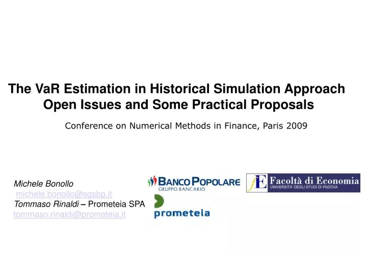
The VaR Estimation in Historical Simulation Approach Open Issues and Some Practical Proposals. Conference on Numerical Methods in Finance, Paris 2009. Michele Bonollo michele.bonollo@sgsbp.it Tommaso Rinaldi – Prometeia SPA tommaso.rinaldi@prometeia.it. Index .

E N D
The VaR Estimation in Historical Simulation Approach Open Issues and Some Practical Proposals Conference on Numerical Methods in Finance, Paris 2009 Michele Bonollo michele.bonollo@sgsbp.it Tommaso Rinaldi – Prometeia SPA tommaso.rinaldi@prometeia.it
Index • PART I Market Risk Mgt and Historical simulation approach • The stylized context vs. the real world context • The challenges of the real world numbers • Historical Simulation approach. Review of the canonical steps • PART II Historical simulation: Open isues, some possible approaches • Issue 1. Scenario P&L. multidimensional full evaluation vs. marginal full evaluation • Issue 2. VaR Estimation. Scenario weighting by l and quantile etimation • Issue 3. Component VaR. Expected return approach vs hybrid parametric approach • PART IIIJust a practical view of the reporting system
Introduction … • Once (3-4 years ago) a (world famous) financial mathematics researcher asked me “What about your work”; I said “I work on market risk, VaR computation”. He said “AgainVaR ? Is is just a quantile …”. While exiting from his University, my feeling was “why so hard to meet theoretical and applied perspective?”. • I do not know the exact answer: in my experience the real world problems are always cross among several fields of knowledge: asset management, financial instruments, financial mathematics, statistics, computation science, regulatory contraints, reporting processes and so on. The theoretical research is (must be) very deep on each task. In the next slides a (vey small) step to take in to account both them
Market Risk Management: stylized view vs. real world • In the usual book description, one has two keys concepts concerning the VaR • The single instrument/position j • The portfolio, i.e. the vector of weights w = (w1, …,wj, …,wN) • The implied underlying idea is that one has to compute the risk measures (VaR, ES, ..) for the whole portoflio, for the single instrument/position, and at most for a few number of subportoflios, following the asset class or other clustering variable
Market Risk Management: stylized view vs. real world • In the actual risk managament process, the portolio is a complex multilevel tree, where the different levels refer to: • The banks of the groups, the types of strategies, the families of products, the risk factors, …..
Historical Simulation approach. The canonical steps • Let • t=1..T the id of scenarios: T = 250, 500 daily • j = 1…N the number of position/instruments • m = (m1…mK) the vector of market paramers underlying • f( ) the pricing functions • The steps are • Collect time series for underlyings/market parameters mt • From data to shocks/returnsst. Compound, or continuous, … • Evaluation of Scenario P&L: PLj,t= fj(mjt + sjt) – fj(mj) • Aggregate scenario P&Ls for the required cluster P&LCt = S … • Estimate the Quantile – VaR or any other risk measure (ES, CVaR, ..)
The challenges of the real world numbers • Some numbers (magnitudes) from our bank, the 4-th in Italy • 100.000 elementary positions, the > 90% derivatives • portfolio tree with 1.000 nodes • 100 billions € of Notional in derivatives • > 1.000 elementary risk factors (IR buckets, underlyings, …) • As concerns the number of variables for which to apply a possible clustering, we have > 10 variables, related to: portfolio/desk, risk factor, product family, issuer/counterparty • Each day, we deliver (at least) 892 “standard” VaR, by .txt file. Moreover the Risk Manager can browse the whole portoflio and to compute the VaR for each required cluster or risk factor (equity, interest, forex) class. The combinations (hypercube D = 10) ∞ • 20 millions of pricing each day: (Instrument x Scenario x RFactor)
Historical Simulation: the basic schema • From the single positions j P&L Deal PTF • … to the cluster P&L • PTF A = Deal1 + Deal2 • (a possible) VaR estimation
Historical Simulation: Canonical algorithm in the IT actual architecture Merlino Risque Money Mate Provider N Bloomberg Reuters Positions Front Office Estrattori MaPaC (1-2) Pricing Prometeia (3) Pricing Sophis (3) Shocks Shocks Pricing Engines Staging Area Export Repository (4) Process 3 Process 1 Clustering Cleaning Process … Process 2 Calcolo HVaR Risk Contributions Calcolo P&L Browsing VaR Computation Reporting QlikView (5)
Issue 1: ScenarioP&L, Full evaluation and marginal Full evaluation • Each day t the market parameters mt move togehter • But, for compliance and strategic views, one often want to decomposte the different sources of risk in a single instrument/portfolio: equity, interest, forex • So the straigh way is to aply marginal shocks stk and then to evaluate the marginal P&Lj,t,k • But P&Lj,t SkP&Lj,t,k • If we suppose that the pricing functions are smooth and follow a taylor representation, it happens because SkP&Lj,t,k consistes of the sum of all the “pure” derivatives, up to ∞, in the taylor expansion, and the interaction terms are lost. Very often the first two terms are enough in the expansion, so the difference is mainly due to the terms ou fo the diagonal in the Hessian matrix of the pricing function • How to “reconciliate” the two measures? We remind the “data oriented” HS schema requires to use a unique large table (millions of rows) and we can not row by row deal with different cases
Issue 1: ScenarioP&L, Full evaluation and marginal Full evaluation The graph below is an example of the difference for a plain vanilla option (SPMIB call) using two different approaches: Full Evaluation and Marginal Full Evaluation. % is small
Issue 1: ScenarioP&L, Full evaluation and marginal Full evaluation Here we have a large, higly exotic portfolio (napoleon, altiplano, rainbow, ..). We poit out that the difference still are quite small
Issue 1: ScenarioP&L, Full evaluation and marginal Full evaluation So what do we do? This interesting hard problem ha fortunately a small impact on computations. So depending from the different situations, we have some different strategies: • For linear or quasi linear portfolio (bond, equity) we can put by definition P&L SUM of marginal P&L • In other cases we take the residual and we split it to the different sources in any way. Consider that this task is very frequent. For example an equity in $ has each day a new value Vt that is Vt = Vt-1 x (1+Rt)(1+FXt), where R anf FX represent the share and the $ return. The interaction effect (R x FX) has to be splitted. The issue is well konwn also in asset management, as “performace contribution – attribution”, see Brinson, Carino, ….
Issue 2: The quantile estimation and scenario weighting by l Here we have to consider a trade off between some different goals: • The quantile estimation, e.g. the simplest empirical quantile (the 5-th worst scenario if T =500, a = 99%), has a high variance behaviour. This is a well known problem in order statistics theory (see David, Huber, ..), but is forgotten from practitioners. • From a risk management perspective, one has to optimize the back testing statistics. In other words, the out of sample P&L that exxcee the ex-ante VaR must be close to the expected frequency. In a 1-year VaR estimation a = 99%, I would expect that only 2.5 times the daily P&L is below the VaR prediction. The accuracy of back testing implies a different capital requiremet by the central bank. If good, the capital requirement is (approximately) 3 times the 10-days 99% VaR • The risk changes over time but it remains unobservable. We can use (see Boudoukh 1996, Finger 2008) also in the non parametric historical simulation approach a l weighting technique à la RiskMetrics. In this case, we weight the probability of scenario before estimating the quantile
Issue 2: The quantile estimation and scenario weighting by l The graph below is an example of VaR calculation using different lambda parameters for a large exotic portfolio “Structured Product”. With l is (now) more conservative • Holding period: 250 day • Confidence level: 99%
Issue 2: The quantile estimation and scenario weighting by l • The VaR of the portfolio has been calculated using different parameters Lambda and is on a portfolio composed of the following indexes: • Nikkey 225 • S&P 500 • EUROSTOXX 50E • The three indexes have the • same weight in the portfolio composition • Holding period: 250 day • Confidence level: 99% The table shows expected and Effective outliers data Portfolio’s Profit & Loss compared with VaR calculated with different Lambda
Issue 2: The quantile estimation and scenario weighting by l • The second exercise of Lambda Weighting was calculated for a portfolio with the followes shares: • IT0001976403 • IT0003856405 • IT0001063210 • IT0001334587 • IT0000072725 • DE0005557508 • DE0005752000 • DE0005140008 • FR0000121261 • This shares have the • same weight in the portfolio composition • Holding period: 401 day • Confidence level: 99% The table shows Expected and Effective outliers data Portfolio’s Profit & Loss compared with VaR calculated with different Lambda
Issue 2: The quantile estimation and scenario weighting by l So what do we do? At now (the project is in progress and fine tuning): • As concerns the high variance of the estimator, the system allows to smooth the system by simple L-estimator, e.g. we do not take the 5-th worst case, but we average in a neighbor. We have not yet applied more sophisticated technique, such as Harrel-Davis estimator (the weight of the scneario is given by its frequency in a bootsrap sampling), Cornish-Fischer and so on. Here, for auditing reasosn and reporting cotraints, converge to simplicity … • As concerns l, from april the “official VaR” is computed with l = 0.98., but each day we compute as a check/warning also the the “plain vanilla” VaR, the is the simplest quantile estimation. Consider that the computation effort is very hard. So we compute 2 x 892 VaR (Portoflio, clustering, …). Each one of them requires: sum of 10.000 100.000 P&L, sort them, estimate VaR. With a 48 (!!) GB RAM server, 20-30 minutes.
Issue 3: Component VaR The additive decomposition of risk is veru useful. In the actual risk management process: • The risk limits are given as VaR limits or greeks limits (delta equivalent, basis point value, vega for 1% shift, ..). The strategic analysis of risk need to split the effect of the different desk / porfolios on the risk: VaR = S … • A good measure is the ComponentVaR (see Garman, Mausser, ..). Using for simplicity the % return notation, not the € P&L notation, if we have a partition of the portoflio indexed by i, the portfolio return is RP, the VaR is R*P, then CVARi E(Ri | VaRP) = E (Ri | RP = R*P) • In the gaussian context, this reduces (see Garman, 96) to CVaRi = R*P x bi x c, b between porfolio and subporfolio • If we apply the definition for the Historical case, if t* is the VaR scenario, we take the P&L for the t* for the subportfolio as CVaRi (see Hallerbach). Nevertheless this simple tecnique may not be used, becaues of high variance, low reliability.
Issue 3: Component VaR Here we see the weakness of the described “pure” non parametric estimation, based of the expectation definition. The portfolio model is of european blue chips, higly correlated (avg r 0.7)
Issue 3: Component VaR A simple robust idea is to “plug-in” the beta-Garman formula in the non parametric approach. We compute b over the T P&L scenario and then fixed the t* VaR-scenario, apply the formula to decompose it. Below the same portfolio, the same compute date. More reliable!
Issue 3: Component VaR The chart below shows VaR Contribution (Component VaR) of each share in portfolio to Total VaR, by appling the hybrid Beta technique over 400 days • The portfolio is composed by the followes shares: • IT0001976403 • IT0003856405 • IT0001063210 • IT0001334587 • IT0000072725 • DE0005557508 • DE0005752000 • DE0005140008 • FR0000121261 • Holding period: 401 days • Confidence level: 99%
Issue 3: Component VaR So what do we do? At now (the project is in progress and fine tuning): • Differently from l, the CVaR is not yet published in the daily reporting, it is computed in order to make software test. • Consider that we could deliver a “number of CVaR” very high (> 1000) depending of all interesting clustering and partitioning of portfolios. • I think we will use hybrid approach or some way very cloe to it. To measure risk is importante, but even more important is that the top management “believes” the the risk meausers. An irregular or “strange” risk measure over time makes is useless
Distribution of the Scenario P&L of a large exotic portfolio
The Tableau de Bord Bank filter Portfolio / Desk
Reporting Historical VaR In relazione a una serie di anomalie “fisiologiche” o determinate da errori del batch Sophis sono èstato messo a punto un sistema di controllo, denominato Outliers, che permette di navigare e visualizzare tali casi: fair value nulli, P&L rilevanti; Le soglie di rilevazione delle anomalie sono parametriche, modificabili dall’utente