Download
1 / 25
270 likes | 459 Views
Statistical Methods for Data Analysis Parameter estimates with RooFit. Luca Lista INFN Napoli. Fits with RooFit. Get data sample (or generate it, for Toy Monte Carlo) Specify data model (PDF’s) Fit specified model to data set with preferred technique (ML, Extended ML, …). Example.

E N D
Statistical Methodsfor Data AnalysisParameter estimateswith RooFit Luca Lista INFN Napoli
Fits with RooFit • Get data sample (or generate it, for Toy Monte Carlo) • Specify data model (PDF’s) • Fit specified model to data set with preferred technique (ML, Extended ML, …) Statistical Methods for Data Analysis
Example RooRealVar x("x","x",-10,10) ; RooRealVar mean("mean","mean of gaussian",0,-10,10); RooRealVar sigma("sigma","width of gaussian",3); RooGaussian gauss("gauss","gaussian PDF",x,mean,sigma); RooDataSet* data = gauss.generate(x,10000); // ML fit is the default gauss.fitTo(*data); mean.Print(); // RooRealVar::mean = // 0.0172335 +/- 0.0299542 sigma.Print(); // RooRealVar::sigma = // 2.98094 +/- 0.0217306 RooPlot* xframe = x.frame(); data->plotOn(xframe); gauss.plotOn(xframe); xframe->Draw(); Further drawing options: pdf.paramOn(xframe,data); data.statOn(xframe); PDFautomaticallynormalizedto dataset Statistical Methods for Data Analysis
Extended ML fits • Specify extended ML fit adding one extra parameter: pdf.fitTo(*data, RooFit::Extended(kTRUE)); Statistical Methods for Data Analysis
Import external data sets • Read a ROOT tree: RooRealVar x(“x”,”x”,-10,10); RooRealVar c(“c”,”c”,0,30); RooDataSet data(“data”,”data”,inputTree, RooArgSet(x,c)); • Automatic removal of entries out of variable range • Read an ASCII file: RooDataSet* data =RooDataSet::read(“ascii.file”, RooArgList(x,c)); • Une line per entry; variable order given by argument list Statistical Methods for Data Analysis
Histogram fits • Use a binned data set: • RooDataHist instead of RooDataSet • Fit with binned model Unbinned Binned RooDataSet RooDataHist RooAbsData Statistical Methods for Data Analysis
Import external histograms • From ROOT TH1/TH2/TH3: RooDataHist bdata1(“bdata”,”bdata”,RooArgList(x),histo1d); RooDataHist bdata2(“bdata”,”bdata”,RooArgList(x,y),histo2d); RooDataHist bdata3(“bdata”,”bdata”,RooArgList(x,y,z),histo3d); • Binning an unbinned data set: RooDataHist* binnedData = data->binnedClone(); • Specifying binning: x.setBins(50); RooDataHist binnedData(“binnedData”, “data”, RooArgList(x), *data); Statistical Methods for Data Analysis
Discrete variables • Define categories • E.g.: b-tag: RooCategory b0flav("b0flav", "B0 flavour"); b0flav.defineType("B0", -1); b0flav.defineType("B0bar", 1); • Several tools defined to combine categories (RooSuperCategory) and analyze data according to categories • See Root user manual for more details… • Switch between PDF’s based on a category can be implemented for simultaneous fits of multiple categories: RooSimultaneous simPdf("simPdf","simPdf", categoryType); simPdf.addPdf(pdfA,"A"); simPdf.addPdf(pdfB,"B"); Indices automatically assignedif omitted Statistical Methods for Data Analysis
Explicit Minuit minimization • Build negative log-Likelihood finction (NLL) // Construct function object representing -log(L) RooNLLVar nll(“nll”, ”nll”, pdf, data); // Minimize nll w.r.t its parameters RooMinuit m(nll); m.migrad(); m.hesse(); • Extra arguments: specify extended likelihood: RooNLLVar nll(“nll”,”nll”,pdf,data,Extended()); • Chi-squared functions (only accepts RooDataHist): RooNLLVar chi2(“chi2”,”chi2”,pdf,data); Statistical Methods for Data Analysis
Drive converging process // Start Minuit session on above nll RooMinuit m(nll); // MIGRAD likelihood minimization m.migrad(); // Run HESSE error analysis m.hesse(); // Set sx to 3, keep fixed in fit sx.setVal(3); sx.setConstant(kTRUE); // MIGRAD likelihood minimization m.migrad(); // Run MINOS error analysis m.minos(); // Draw 1,2,3 ‘sigma’ contours in sx,sy m.contour(sx, sy); Statistical Methods for Data Analysis
Minuit function MIGRAD Purpose: find minimum Progress information,watch for errors here ********** ** 13 **MIGRAD 1000 1 ********** (some output omitted) MIGRAD MINIMIZATION HAS CONVERGED. MIGRAD WILL VERIFY CONVERGENCE AND ERROR MATRIX. COVARIANCE MATRIX CALCULATED SUCCESSFULLY FCN=257.304 FROM MIGRAD STATUS=CONVERGED 31 CALLS 32 TOTAL EDM=2.36773e-06 STRATEGY= 1 ERROR MATRIX ACCURATE EXT PARAMETER STEP FIRST NO. NAME VALUE ERROR SIZE DERIVATIVE 1 mean 8.84225e-023.23862e-01 3.58344e-04 -2.24755e-02 2 sigma 3.20763e+002.39540e-01 2.78628e-04 -5.34724e-02 ERR DEF= 0.5 EXTERNAL ERROR MATRIX. NDIM= 25 NPAR= 2 ERR DEF=0.5 1.049e-01 3.338e-04 3.338e-04 5.739e-02 PARAMETER CORRELATION COEFFICIENTS NO. GLOBAL 1 2 1 0.00430 1.000 0.004 2 0.00430 0.004 1.000 Parameter values and approximate errors reported by MINUIT Error definition (in this case 0.5 for a likelihood fit) Statistical Methods for Data Analysis
Minuit function MIGRAD Purpose: find minimum Value of c2 or likelihood at minimum (NB: c2 values are not divided by Nd.o.f) ********** ** 13 **MIGRAD 1000 1 ********** (some output omitted) MIGRAD MINIMIZATION HAS CONVERGED. MIGRAD WILL VERIFY CONVERGENCE AND ERROR MATRIX. COVARIANCE MATRIX CALCULATED SUCCESSFULLY FCN=257.304 FROM MIGRAD STATUS=CONVERGED 31 CALLS 32 TOTAL EDM=2.36773e-06 STRATEGY= 1 ERROR MATRIX ACCURATE EXT PARAMETER STEP FIRST NO. NAME VALUE ERROR SIZE DERIVATIVE 1 mean 8.84225e-02 3.23862e-01 3.58344e-04 -2.24755e-02 2 sigma 3.20763e+00 2.39540e-01 2.78628e-04 -5.34724e-02 ERR DEF= 0.5 EXTERNAL ERROR MATRIX. NDIM= 25 NPAR= 2 ERR DEF=0.5 1.049e-01 3.338e-04 3.338e-04 5.739e-02 PARAMETER CORRELATION COEFFICIENTS NO. GLOBAL 1 2 1 0.00430 1.000 0.004 2 0.00430 0.004 1.000 Approximate Error matrix And covariance matrix Statistical Methods for Data Analysis
Minuit function MIGRAD Purpose: find minimum Status: Should be ‘converged’ but can be ‘failed’ Estimated Distance to Minimumshould be small O(10-6) Error Matrix Qualityshould be ‘accurate’, but can be ‘approximate’ in case of trouble ********** ** 13 **MIGRAD 1000 1 ********** (some output omitted) MIGRAD MINIMIZATION HAS CONVERGED. MIGRAD WILL VERIFY CONVERGENCE AND ERROR MATRIX. COVARIANCE MATRIX CALCULATED SUCCESSFULLY FCN=257.304 FROM MIGRAD STATUS=CONVERGED 31 CALLS 32 TOTAL EDM=2.36773e-06 STRATEGY= 1 ERROR MATRIX ACCURATE EXT PARAMETER STEP FIRST NO. NAME VALUE ERROR SIZE DERIVATIVE 1 mean 8.84225e-02 3.23862e-01 3.58344e-04 -2.24755e-02 2 sigma 3.20763e+00 2.39540e-01 2.78628e-04 -5.34724e-02 ERR DEF= 0.5 EXTERNAL ERROR MATRIX. NDIM= 25 NPAR= 2 ERR DEF=0.5 1.049e-01 3.338e-04 3.338e-04 5.739e-02 PARAMETER CORRELATION COEFFICIENTS NO. GLOBAL 1 2 1 0.00430 1.000 0.004 2 0.00430 0.004 1.000 Statistical Methods for Data Analysis
Minuit function HESSE Purpose: calculate error matrix from ********** ** 18 **HESSE 1000 ********** COVARIANCE MATRIX CALCULATED SUCCESSFULLY FCN=257.304 FROM HESSE STATUS=OK 10 CALLS 42 TOTAL EDM=2.36534e-06 STRATEGY= 1 ERROR MATRIX ACCURATE EXT PARAMETER INTERNAL INTERNAL NO. NAME VALUE ERROR STEP SIZE VALUE 1 mean 8.84225e-02 3.23861e-01 7.16689e-05 8.84237e-03 2 sigma 3.20763e+00 2.39539e-01 5.57256e-05 3.26535e-01 ERR DEF= 0.5 EXTERNAL ERROR MATRIX. NDIM= 25 NPAR= 2 ERR DEF=0.5 1.049e-01 2.780e-04 2.780e-04 5.739e-02 PARAMETER CORRELATION COEFFICIENTS NO. GLOBAL 1 2 1 0.003581.000 0.004 2 0.003580.004 1.000 Symmetric errors calculated from 2nd derivative of –ln(L) or c2 Statistical Methods for Data Analysis
Minuit function HESSE Purpose: calculate error matrix from ********** ** 18 **HESSE 1000 ********** COVARIANCE MATRIX CALCULATED SUCCESSFULLY FCN=257.304 FROM HESSE STATUS=OK 10 CALLS 42 TOTAL EDM=2.36534e-06 STRATEGY= 1 ERROR MATRIX ACCURATE EXT PARAMETER INTERNAL INTERNAL NO. NAME VALUE ERROR STEP SIZE VALUE 1 mean 8.84225e-02 3.23861e-01 7.16689e-05 8.84237e-03 2 sigma 3.20763e+00 2.39539e-01 5.57256e-05 3.26535e-01 ERR DEF= 0.5 EXTERNAL ERROR MATRIX. NDIM= 25 NPAR= 2 ERR DEF=0.5 1.049e-01 2.780e-04 2.780e-04 5.739e-02 PARAMETER CORRELATION COEFFICIENTS NO. GLOBAL 1 2 1 0.00358 1.000 0.004 2 0.003580.004 1.000 Error matrix (Covariance Matrix) calculated from Statistical Methods for Data Analysis
Minuit function HESSE Purpose: calculate error matrix from ********** ** 18 **HESSE 1000 ********** COVARIANCE MATRIX CALCULATED SUCCESSFULLY FCN=257.304 FROM HESSE STATUS=OK 10 CALLS 42 TOTAL EDM=2.36534e-06 STRATEGY= 1 ERROR MATRIX ACCURATE EXT PARAMETER INTERNAL INTERNAL NO. NAME VALUE ERROR STEP SIZE VALUE 1 mean 8.84225e-02 3.23861e-01 7.16689e-05 8.84237e-03 2 sigma 3.20763e+00 2.39539e-01 5.57256e-05 3.26535e-01 ERR DEF= 0.5 EXTERNAL ERROR MATRIX. NDIM= 25 NPAR= 2 ERR DEF=0.5 1.049e-01 2.780e-04 2.780e-04 5.739e-02 PARAMETER CORRELATION COEFFICIENTS NO. GLOBAL 1 2 1 0.003581.000 0.004 2 0.003580.004 1.000 Correlation matrix rijcalculated from Statistical Methods for Data Analysis
Minuit function HESSE Purpose: calculate error matrix from ********** ** 18 **HESSE 1000 ********** COVARIANCE MATRIX CALCULATED SUCCESSFULLY FCN=257.304 FROM HESSE STATUS=OK 10 CALLS 42 TOTAL EDM=2.36534e-06 STRATEGY= 1 ERROR MATRIX ACCURATE EXT PARAMETER INTERNAL INTERNAL NO. NAME VALUE ERROR STEP SIZE VALUE 1 mean 8.84225e-02 3.23861e-01 7.16689e-05 8.84237e-03 2 sigma 3.20763e+00 2.39539e-01 5.57256e-05 3.26535e-01 ERR DEF= 0.5 EXTERNAL ERROR MATRIX. NDIM= 25 NPAR= 2 ERR DEF=0.5 1.049e-01 2.780e-04 2.780e-04 5.739e-02 PARAMETER CORRELATION COEFFICIENTS NO. GLOBAL 1 2 1 0.003581.000 0.004 2 0.003580.004 1.000 Global correlation vector:correlation of each parameter with all other parameters Statistical Methods for Data Analysis
Minuit function MINOS Error analysis through Dnll contour finding ********** ** 23 **MINOS 1000 ********** FCN=257.304 FROM MINOS STATUS=SUCCESSFUL 52 CALLS 94 TOTAL EDM=2.36534e-06 STRATEGY= 1 ERROR MATRIX ACCURATE EXT PARAMETER PARABOLICMINOS ERRORS NO. NAME VALUE ERROR NEGATIVE POSITIVE 1 mean 8.84225e-02 3.23861e-01-3.24688e-01 3.25391e-01 2 sigma 3.20763e+00 2.39539e-01 -2.23321e-01 2.58893e-01 ERR DEF= 0.5 Symmetric error(repeated result from HESSE) MINOS errorCan be asymmetric(in this example the ‘sigma’ error is slightly asymmetric) Wouter Verkerke, NIKHEF Statistical Methods for Data Analysis
Mitigating fit stability problems Strategy I – More orthogonal choice of parameters Example: fitting sum of 2 Gaussians of similar width HESSE correlation matrix PARAMETER CORRELATION COEFFICIENTS NO. GLOBAL [ f] [ m] [s1] [s2] [ f] 0.96973 1.000 -0.135 0.9180.915 [ m] 0.14407 -0.135 1.000 -0.144 -0.114 [s1] 0.92762 0.918 -0.144 1.000 0.786 [s2] 0.92486 0.915 -0.114 0.786 1.000 Widths s1,s2strongly correlatedfraction f Statistical Methods for Data Analysis
Mitigating fit stability problems Different parameterization: Correlation of width s2 and fraction f reduced from 0.92 to 0.68 Choice of parameterization matters! Strategy II – Fix all but one of the correlated parameters If floating parameters are highly correlated, some of them may be redundant and not contribute to additional degrees of freedom in your model PARAMETER CORRELATION COEFFICIENTS NO. GLOBAL [f] [m] [s1] [s2] [ f] 0.96951 1.000 -0.134 0.917 -0.681 [ m] 0.14312 -0.134 1.000 -0.143 0.127 [s1] 0.98879 0.917 -0.143 1.000 -0.895 [s2] 0.96156 -0.681 0.127 -0.895 1.000 Statistical Methods for Data Analysis
Fit stability with polynomials Warning: Regular parameterization of polynomials a0+a1x+a2x2+a3x3nearly always results in strong correlations between the coefficients ai. Fit stability problems, inability to find right solution common at higher orders Solution: Use existing parameterizations of polynomials that have (mostly) uncorrelated variables Example: Chebychev polynomials Statistical Methods for Data Analysis
Browsing fit results As fits grow in complexity (e.g. 45 floating parameters), number of output variables increases Need better way to navigate output that MINUIT screen dump RooFitResult holds complete snapshot of fit results Constant parameters Initial and final values of floating parameters Global correlations & full correlation matrix Returned from RooAbsPdf::fitTo() when “r” option is supplied Compact & verbose printing mode Compact Mode Constantparametersomitted incompact mode fitres->Print() ; RooFitResult: min. NLL value: 1.6e+04, est. distance to min: 1.2e-05 Floating Parameter FinalValue +/- Error -------------------- -------------------------- argpar -4.6855e-01 +/- 7.11e-02 g2frac 3.0652e-01 +/- 5.10e-03 mean1 7.0022e+00 +/- 7.11e-03 mean2 1.9971e+00 +/- 6.27e-03 sigma 2.9803e-01 +/- 4.00e-03 Alphabetical parameter listing Statistical Methods for Data Analysis
Browsing fit results Verbose printing mode fitres->Print(“v”) ; RooFitResult: min. NLL value: 1.6e+04, est. distance to min: 1.2e-05 Constant Parameter Value -------------------- ------------ cutoff 9.0000e+00 g1frac 3.0000e-01 Floating Parameter InitialValue FinalValue +/- Error GblCorr. -------------------- ------------ -------------------------- -------- argpar -5.0000e-01 -4.6855e-01 +/- 7.11e-02 0.191895 g2frac 3.0000e-01 3.0652e-01 +/- 5.10e-03 0.293455 mean1 7.0000e+00 7.0022e+00 +/- 7.11e-03 0.113253 mean2 2.0000e+00 1.9971e+00 +/- 6.27e-03 0.100026 sigma 3.0000e-01 2.9803e-01 +/- 4.00e-03 0.276640 Constant parameterslisted separately Initial,final value and global corr. listed side-by-side Correlation matrix accessed separately Statistical Methods for Data Analysis
Browsing fit results Easy navigation of correlation matrix Select single element or complete row by parameter name RooFitResult persistable with ROOT I/O Save your batch fit results in a ROOT file and navigateyour results just as easy afterwards fitres->correlation("argpar","sigma") (const Double_t)(-9.25606412005910845e-02) fitres->correlation("mean1")->Print("v") RooArgList::C[mean1,*]: (Owning contents) 1) RooRealVar::C[mean1,argpar] : 0.11064 C 2) RooRealVar::C[mean1,g2frac] : -0.0262487 C 3) RooRealVar::C[mean1,mean1] : 1.0000 C 4) RooRealVar::C[mean1,mean2] : -0.00632847 C 5) RooRealVar::C[mean1,sigma] : -0.0339814 C Statistical Methods for Data Analysis
References • RooFit online tutorial • http://roofit.sourceforge.net/docs/tutorial/index.html • Credits: • RooFit slides and examples extracted, adapted and/or inspired by original presentations by Wouter Verkerke Statistical Methods for Data Analysis