CONSTITUTIVE equation of hyperelastic materials identified by inflation test

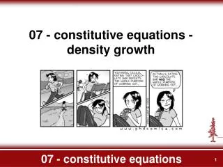
1. EXPERIMENTAL METHODS 2010 PROJECT CONSTITUTIVE EQUATIONS CONSTITUTIVE equation of hyperelastic materials identified by inflation test Motivation Advanced experimental techniques (laser scanner, confocal probe) How to describe mechanical properties of biological materials? Using MATLAB for identification of a mathematical model. Task prepared within the project FRVS 90/2010

2. EXPERIMENTAL METHODS 2010 PROJECT CONSTITUTIVE EQUATIONS Laser scanner Microscan or confocal probe Aim of project: Identify mechanical properties (elasticity) of vascular tissue. Tested sample is a tube (artery, vein,…) loaded by inner pressure and by axial force. Recorded inflation and extension will be used for a simple constitutive model identification.

3. EXPERIMENTAL METHODS 2010 PROJECT CONSTITUTIVE EQUATIONS "Dogbone" sample Constitutive equation of hyperelastic solids Constitutive equations (relationships between stresses and kinematics) are usually designed in a different way for different materials: one class is represented by metals, crystals,… where arrays of atoms held together by interatomic forces (elastic stretches can be of only few percents). The second class are polymeric materials (biomaterials) characterized by complicated 3D networks of long-chain macromolecules with freely rotating links – interlocking is only at few places (cross-links). In this case the stretches can be much greater (of the order of tens or hundreds percents) and their behavior is highly nonlinear. Both the deformations (kinematics of deformed material, will be recorded by laser scanner and confocal probe) and stresses (evaluated from pressure and axial load) are characterized by tensors of the second order. Deformation is different in different directions (axial/radial/peripheral stretches) and also stresses differ (axial/radial/peripheral stresses). This is why it is necessary to use tensors.

4. EXPERIMENTAL METHODS 2010 PROJECT CONSTITUTIVE EQUATIONS z loaded configuration t R r r reference configuration Deformation tensor F transforms a vector of a material segment from reference configuration to loaded configuration. Special case - thick wall cylinder tr and z are principal stretches (stretches in the principal directions). There are always three principal direction characterized by the fact that a material segment is not rotated, but only extended (by the stretch ratio). In this specific case and when the pipe is loaded only by inner pressure and by axial force, there is no twist and the principal directions are identical with directions of axis of cylindrical coordinate system. In this case the deformation gradient has simple diagonal form

5. EXPERIMENTAL METHODS 2010 PROJECT CONSTITUTIVE EQUATIONS Cauchy Green tensor C Disadvantage of deformation gradient F - it includes a rigid body rotation. And this rotation cannot effect the stress state (rotation is not a deformation). The rotation is excluded in the right Cauchy Green tensor C defined as Stress state can be expressed in terms of Cauchy Green tensor. Each tensor of the second order can be characterized by three scalars independent of coordinate system (mention the fact that if you change coordinate system all matrices F,C will be changed). The first two invariants (they characterize “magnitudes” of tensor) are defined as Material of blood vessel walls can be considered incompressible, therefore the volume of a loaded part is the same as the volume in the unloaded reference state. Ratio of volumes can be expressed in terms of stretches (unit cube is transformed to the brick having sides t r z) Therefore only two stretches are independent and invariants of C-tensor can be expressed only in terms of these two independent (and easily measurable) stretches

6. EXPERIMENTAL METHODS 2010 PROJECT CONSTITUTIVE EQUATIONS t z Mooney Rivlin model Using invariants it is possible to suggest several different models defining energy of deformation W (energy related to unit volume – this energy has unit of stress, Pa) Example: Mooney Rivlin model of hyperelastic material Remark: for an unload sample are all stretches 1 (t =r = z=1) and Ic=3, IIc=3, therefore deformation energy is zero (as it should be). Stresses are partial derivatives of deformation energy W with respect stretches (please believe it wihout proof) These equations represent constitutive equation, model calculating stresses for arbitrary stretches and for given coefficients c1, c2. At unloaded state with unit stretches, the stresses are zero (they represent only elastic stresses and an arbitrary isotropic hydrostatic pressure can be added giving total stresses).

7. EXPERIMENTAL METHODS 2010 PROJECT CONSTITUTIVE EQUATIONS G-force r0 h p z Evaluation of stretches and stresses Only two stretches is to be evaluated from measured outer radius after and before loading ro, Ro, frominitial wall thickness H, and lengths of sample l after and L before loading. This is quadratic equation Therefore it is sufficient to determine Ro,H,L before measurement and only outer radius ro and length l after loading, so that the kinematics of deformation is .fully described. Corresponding stresses can be derived from balance of forces acting upon annular and transversal cross section of pipe t

8. EXPERIMENTAL METHODS 2010 PROJECT CONSTITUTIVE EQUATIONS Identification of model parameters c1,c2 Optimal parameters can be identified by comparison measured stresses with stresses predicted by constitutive equations Criterion of sum of squares of differences should be minimized i-index of experiment w-weight of axial stresses differences Minimum of S exists at the point where both partial derivatives of S with respect to c1, c2 are zero

9. EXPERIMENTAL METHODS 2010 PROJECT CONSTITUTIVE EQUATIONS Identification of model parameters c1,c2 , accuracy Result is the following system of two linear algebraic equations In matrix notation Ac=b These equations can be easily solved for example by Cramer’s rule or by inversion of matrix A. Inverted matrix A (covariance matrix) enables to calculate confidence intervals or standard deviation of calculated parameters c1,c2 as Special case zero pressure represents a constraint between s (t=0) This is only an approximation that is to be used as soon as only one (axial) stretch is measured. Anyway, regression analysis has to be carried out iteratively based upon estimates of c1, c2.

10. EXPERIMENTAL METHODS 2010 PROJECT CONSTITUTIVE EQUATIONS MATLAB programming Previous analysis can be implemented in form of MATLAB M-files Data with both axial and circumferential stretches Data only axial stretches delta_l=load('delta_l.txt') lambda_z=(70+delta_l)/70 delta_r=load('delta_r.txt') lambda_t=(5.46+delta_r)/5.46 p=load('p.txt') sigma_t=p.*(5.46.*lambda_t.*lambda_z./0.6807-1/2) sigma_z=sigma_t./2+0.*lambda_z./(3.14*0.6807*(2*5.46-0.6807)) i=1 for i=1:length(lambda_z) A_t=lambda_t(i).^2-1./(lambda_t(i).^2.*lambda_z(i).^2) A_z=lambda_z(i).^2-1./(lambda_t(i).^2.*lambda_z(i).^2) B_t=lambda_t(i).^2.*lambda_z(i).^2-1./(lambda_t(i).^2) B_z=lambda_t(i).^2.*lambda_z(i).^2-1./(lambda_z(i).^2) C=[A_t,B_t;A_z,B_z] K=[sigma_t(i)./2;sigma_z(i)./2] c(:,i)=[C\K] i=i+1 end a=load('f_g,delta_l.txt') lambda_z=(70+a(:,2))/70 lambda_t=sqrt(1./lambda_z) %lambda_t=nthroot((2*0.1./(lambda_z.^2)-0.02)./(2.*0.1-0.02.*lambda_z.^2),4) sigma_t=[0,0,0,0,0,0]' sigma_z=sigma_t./2+a(:,1).*lambda_z./(3.14*0.6807*(2*5.46-0.6807)) i=1 for i=1:length(lambda_z) A_t=lambda_t(i).^2-1./(lambda_t(i).^2.*lambda_z(i).^2) A_z=lambda_z(i).^2-1./(lambda_t(i).^2.*lambda_z(i).^2) B_t=lambda_t(i).^2.*lambda_z(i).^2-1./(lambda_t(i).^2) B_z=lambda_t(i).^2.*lambda_z(i).^2-1./(lambda_z(i).^2) C=[A_t,B_t;A_z,B_z] K=[sigma_t(i)./2;sigma_z(i)./2] c(:,i)=[C\K] i=i+1 end c=c'

11. EXPERIMENTAL METHODS 2010 PROJECT CONSTITUTIVE EQUATIONS • What is measured • Axial displacement (confocal probe 1) • Radial displacement prifile (laser scanner) • Pressure (strain gauge transducer Cresto) • Deformation of surface by cross correlation (optionally) • Twist of sample (confocal probe)-just only for checking of irregularities (twist should be zero for perfectly symmetric sample and loading) EXPERIMENT Laboratory if cardiovascular systems Laser scanner Tested tube Confocal probes 1500N N cross correlation inflatation confocal probes for a twist of loaded sample measurement load cell strain gauges laser scanner axial load

12. EXPERIMENTAL METHODS 2010 PROJECT CONSTITUTIVE EQUATIONS EXPERIMENT Time profile data synchronization from Pressure transducer/Laser scanner/Confocal probes Laser scanner: is it triggered at up or down edge? Write a MATLAB program deciding (by comparing maxima and minima in the series of pulses) whether the recording of laser scanner data are triggered by the leading or the trailing edge of green button.

13. EXPERIMENTAL METHODS 2010 PROJECT CONSTITUTIVE EQUATIONS EXPERIMENT Transversal profile from laser scanner: how to evaluate radius of inflated pipe 3 points define a circle. So you can evaluate triplets (for n=100 this is 161700 radii) and estimate radius by average. y x0 y0 x3 y3 x1 y1 Please, check it I probably made an error in the expressions x2 y2 x

14. EXPERIMENTAL METHODS 2010 PROJECT CONSTITUTIVE EQUATION LABORATORY REPORT • Front page: Title, authors, date • Content, list of symbols • Introduction, aims of project, references • Description of experimental setup • Geometry of samples (D,L,h, basic statistics) • Elongation at atmospheric pressure (6 different weights, axial motion recorded visually and by confocal probe). Table. • Inflation at specific axial load and variable pressure (radial displacement evaluated by laser scanner, axial displacement by confocal probe). Graph of typical radial profile. Recorded data attached in files. • Evaluation of recorded data by Matlab. Results (c1,c2 evaluated from extension test and from inflation test) in table. • Graph: Radial displacement versus pressure (experimental results-points, model prediction by continuous line). • Conclusion (identify interesting results and problems encountered)