Download
1 / 36
370 likes | 389 Views
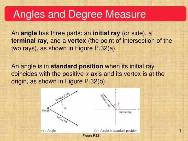
Angles and Degree Measure. An angle has three parts: an initial ray (or side), a terminal ray, and a vertex (the point of intersection of the two rays), as shown in Figure P.32(a).

E N D
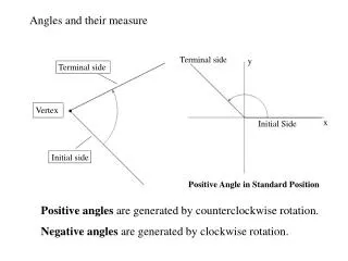
Angles and Degree Measure An angle has three parts: an initial ray (or side), a terminal ray, and a vertex (the point of intersection of the two rays), as shown in Figure P.32(a). An angle is in standard position when its initial ray coincides with the positive x-axis and its vertex is at the origin, as shown in Figure P.32(b). Figure P.32
Angles and Degree Measure It is assumed that you are familiar with the degree measure of an angle.It is common practice to use (the lowercase Greek letter theta) to represent both an angle and its measure. Angles between 0° and 90° are acute, and angles between 90° and 180° are obtuse.
Angles and Degree Measure Positive angles are measured counterclockwise, and negative angles are measured clockwise. For instance, Figure P.33 shows an angle whose measure is −45°. Figure P.33
Angles and Degree Measure You cannot assign a measure to an angle by simply knowing where its initial and terminal rays are located. To measure an angle, you must also know how the terminal ray was revolved. For example, Figure P.33 shows that the angle measuring −45° has the same terminal ray as the angle measuring 315°. Such angles are coterminal. In general, if is any angle, then + n(360), n is a nonzero integer, is coterminal with .
Angles and Degree Measure An angle that is larger than 360° is one whose terminal ray has been revolved more than one full revolution counterclockwise, as shown in Figure P.34(a). You can form an angle whose measure is less than −360° by revolving a terminal ray more than one full revolution clockwise, as shown in Figure P.34(b). Figure P.34
Radian Measure To assign a radian measure to an angle , consider to bea central angle of a circle of radius 1, as shown in Figure P.35. The radian measure of is then defined to be the length of the arc of the sector. Because the circumference of a circle is 2r, the circumference of a unit circle (of radius 1) is 2. Figure P.35
Radian Measure This implies that the radian measure of an angle measuring 360° is 2. In other words, 360° = 2radians. Using radian measure for , the length s of a circular arc of radius r is s = r, as shown in Figure P.36. Figure P.36
Radian Measure You should know the conversions of the common angles shown in Figure P.37. For other angles, use the fact that 180° is equal to radians. Radian and degree measures for several common angles Figure P.37
The Trigonometric Functions There are two common approaches to the study of trigonometry. In one, the trigonometric functions are defined as ratios of two sides of a right triangle. In the other, these functions are defined in terms of a point on the terminal ray of an angle in standard position. The six trigonometric functions, sine, cosine, tangent, cotangent, secant, and cosecant (abbreviated as sin, cos, tan, cot, sec, and csc, respectively), are defined from both viewpoints.
The Trigonometric Functions Figure P.39 Figure P.38
The Trigonometric Functions The trigonometric identities listed below are direct consequences of the definitions.
EvaluatingTrigonometric Functions There are two ways to evaluate trigonometric functions: • decimal approximations with a graphing utility and • exact evaluations using trigonometric identities and formulas from geometry. When using a graphing utility to evaluate a trigonometric function, remember to set the graphing utility to the appropriate mode—degree mode or radian mode.
Example 2 – Exact Evaluation of Trigonometric Functions Evaluate the sine, cosine, and tangent of /3. Solution: Because 60° = /3 radians, you can draw an equilateral triangle with sides of length1 and as one of its angles, as shown in Figure P.40. Because the altitude of this triangle bisects its base, you know that Figure P.40
Example 2 – Solution cont’d Using the Pythagorean Theorem, you obtain, Now, knowing the values of x, y, and r, you can write the following.
EvaluatingTrigonometric Functions The degree and radian measures of several common angles are shown in the table below, along with the corresponding values of the sine, cosine, and tangent
EvaluatingTrigonometric Functions See Figure P.41. Figure P.41
EvaluatingTrigonometric Functions The quadrant signs for the sine, cosine, and tangent functions are shown in Figure P.42. Figure P.42
EvaluatingTrigonometric Functions To find the angles in quadrants other than the first quadrant, you can use the concept of a reference angle (see Figure P.43), with the appropriate quadrant sign. Figure P.43
EvaluatingTrigonometric Functions For instance, the reference angle for 3/4 is /4, and because the sine is positive in Quadrant II, you can write Similarly, because the reference angle for 330° is 30°, and the tangent is negative in Quadrant IV, you can write
Solving Trigonometric Equations How would you solve the equation sin= 0? You know that = 0 is one solution, but this is not the only solution. Any one of the following values of is also a solution. You can write this infinite solution set as {n: n is an integer}.
Example 4 – Solving a Trigonometric Equation Solve the equation Solution: To solve the equation, you should consider that the sine function is negative in Quadrants III and IV and that So, you are seeking values of in the third and fourth quadrants that have a reference angle of /3.
Example 4 – Solution cont’d In the interval [0, 2], the two angles fitting these criteria are, By adding integer multiples of 2to each of these solutions, you obtain the following general solution.
Example 4 – Solution cont’d See Figure P.44. Figure P.44
Graphs of Trigonometric Functions A function f is periodic when there exists a positive real number p such that f(x + p) = f(x) for all x in the domain of f. The least such positive value of p is the period of f. The sine, cosine, secant, and cosecant functions each have a period of 2, and the other two trigonometric functions, tangent and cotangent, have a period of , as shown in Figure P.45.
Graphs of Trigonometric Functions The graphs of the six trigonometric functions Figure P.45
Graphs of Trigonometric Functions Note in Figure P.45 that the maximum value of sin x and cos x is 1 and the minimum value is −1. The graphs of the functions y = a sin bx and y = a cos bx oscillate between −a and a, and so have an amplitude of |a|. Furthermore, because bx = 0 when x = 0 and bx = 2when x = 2/b, it follows that the functions y = a sin bx and y = a cos bx each have a period of 2/|b|.
Graphs of Trigonometric Functions The table below summarizes the amplitudes and periods of some types of trigonometric functions.
Example 6 – Sketching the Graph of a Trigonometric Function Sketch the graph of f(x) = 3 cos 2x. Solution: The graph of f(x) = 3 cos 2x has an amplitude of 3 and a period of 2/2 = . Using the basic shape of the graph of the cosine function, sketch one period of the function on the interval [0, ], using the following pattern.
Example 6 – Solution cont’d By continuing this pattern, you can sketch several cycles of the graph, as shown in Figure P.46. Figure P.46
Example 7 – Shifts of Graphs of Trigonometric Functions a. To sketch the graph of f(x) = sin(x + /2), shift the graph of y = sin x to the left /2 units, as shown in Figure P.47(a). Transformations of the graph of y = sin x Figure P.47
Example 7 – Shifts of Graphs of Trigonometric Functions cont’d b. To sketch the graph of f(x) = 2 + sin x, shift the graph of y = sin x upward two units, as shown in Figure P.47(b). Transformations of the graph of y = sin x Figure P.47
Example 7 – Shifts of Graphs of Trigonometric Functions cont’d c. To sketch the graph of f(x) = 2 + sin(x − /4), shift the graph of y = sin x upward two units and to the right /4 units, as shown in Figure P.47(c). Transformations of the graph of y = sin x Figure P.47