Download
1 / 16
160 likes | 240 Views
Recall Lecture 10. DC analysis of BJT BE Loop (EB Loop) – V BE for npn and V EB for pnp CE Loop (EC Loop) - V CE for npn and V EC for pnp. I E. EXAMPLE - PNP. Given = 75 and V EC = 6V. Find the values of the labelled parameters, R C and I E,. DC analysis of BJT

E N D
Recall Lecture 10 • DC analysis of BJT • BE Loop (EB Loop) – VBE for npn and VEB for pnp • CE Loop (EC Loop) - VCE for npn and VEC for pnp
IE EXAMPLE - PNP Given = 75 and VEC = 6V. Find the values of the labelled parameters, RC and IE,
DC analysis of BJT • When node voltages is known, branch current equations can be used. (Va – Vb) / R = I R b a I
BJT Circuits at DC = 0.99 KVL at BE loop: 0.7 + IERE – 4 = 0 IE = 3.3 / 3.3 = 1 mA Hence, IC = IE= 0.99 mA IB = IE – IC = 0.01 mA KVL at CE loop: ICRC + VCE + IERE – 10 = 0 VCE = 10 – 3.3 – 4.653 = 2.047 V
BJT Circuits at DC = 0.99 VC = 5.347 V Hence, VCE = VC – VE = 5.347 – 3.3 = 2.047 V IC = IE IB = IE - IC VBE = 0.7V VB – VE = 0.7V VE = 4 – 0.7 = 3.3 V since VB = 4V VE – 0 = IE 10 - VC = IC 3.3 k 4.7 k
Load Lineand Voltage Transfer Characteristic can be used to visualize the characteristic of the transistor circuits.
Input Load Line – IB versus VBE Derived using B-E loop • The input load line is obtained from Kirchhoff’s voltage law equation around the B-E loop, written as follows: VBE – VBB + IBRB = 0 • Both the load line and the quiescent base current change as either or both VBBand RB change.
IB = -VBE + 4 220k 220k For example; • The input load line is essentially the same as the load line characteristics for diode circuits. VBE – 4 + IB(220k)= 0 y = mx + c • IBQ = 15 μA
Output Load Line – IC versus VCE Derived using C-E loop • For the C-E portion of the circuit, the load line is found by writing Kirchhoff’s voltage law around the C-E loop. We obtain:
IC = -VCE + 10 2k 2k For example; y = mx + c • To find the intersection points setting IC= 0, VCE = VCC = 10 V • setting VCE = 0 IC= VCC / RC = 5 mA Q-point is the intersection of the load line with the iCvsvCE curve, corresponding to the appropriate base current
Example: Calculation and Load Line Calculate the characteristics of a circuit containing an emitter resistor and plot the output load line. For the circuit, let VBE(on) = 0.7 V and β = 75.
Load Line Use KVL at B-E loop
VCE = 12 – IC (1.01) IC = - VCE + 12 1.01 IB = 75.1 A VCE = 12 – 5.63 (1.01) VCE = 6.31 V