Download
1 / 37
440 likes | 708 Views
Lecture 3 Taylor Series Expansion. Inline function Taylor series Matlab codes for Taylor series expansion. inline function. How to create a function ? Such as f(x)=sin(x)*cos(x) Two steps for creation of an inline function Get a string for representing a valid expression

E N D
Lecture 3 Taylor Series Expansion • Inline function • Taylor series • Matlab codes for Taylor series expansion 數值方法2008, Applied Mathematics NDHU
inline function • How to createa function ? • Such as f(x)=sin(x)*cos(x) • Two steps for creation of an inline function • Get a string for representing a valid expression • Apply inline.m to translate a string to an inline function 數值方法2008, Applied Mathematics NDHU
>> g=inline('x^2+1') g = Inline function: g(x) = x^2+1 >> g(2) ans = 5 數值方法2008, Applied Mathematics NDHU
>> g=inline('x^2+1') g = Inline function: g(x) = x^2+1 >> g(2) ans = 5 數值方法2008, Applied Mathematics NDHU
Function plot • Get a string for representing an expression • Apply inline.m to translate a string to an inline function • Apply linspace.m to form a linear partition to [-5 5] • Determine function outputs of all elements in a partition vector • Plot a figure for given function 數值方法2008, Applied Mathematics NDHU
Input a string, fs f=inline(fs) Use ‘inline’ to generatean inline function x=linspace(-5,5) form a uniform partition to [-5 5] y=f(x) plot(x,y) 數值方法2008, Applied Mathematics NDHU
Demo Source codes % This example illustrates creation % of an inline function fprintf('input a string to specify a desired fun\n'); fs=input(‘ex. x.^2+2*x+1:','s'); f=inline(fs); range=5; x=-range:0.01:range; y=f(x); plot(x,y); 數值方法2008, Applied Mathematics NDHU
cos(x) 數值方法2008, Applied Mathematics NDHU
Input a string, fs f=inline(fs) N=800;d=2; A=rand(2,N); x=A(1,:); y=A(2,:); z=f(x1,x2) plot3(x,y, z, '. ') 數值方法2008, Applied Mathematics NDHU
A sample from function surface f(x,y)=x.^2+3*y.^2 數值方法2008, Applied Mathematics NDHU
Demo Source codes % Inline function creation % The created inline function has two input arguments % Plot a sample from the function surface fs='x.^2+3*y.^2'; f=inline(fs); a=rand(2,800)*2-1; x=a(1,:);y=a(2,:); z=f(x,y); plot3(x,y,z,'.'); 數值方法2008, Applied Mathematics NDHU
3d plot 3D plot t = 0:pi/50:10*pi; plot3(sin(t),cos(t),t); 數值方法2008, Applied Mathematics NDHU
x=linspace(0,1); mesh x=linspace(-1,1); y=linspace(-1,1)'; X=repmat(x,100,1); Y=repmat(y,1,100); Z=X.^2+Y.^2 mesh(x,y,Z) 數值方法2008, Applied Mathematics NDHU
surface x=linspace(-1,1); y=linspace(-1,1)'; X=repmat(x,100,1); Y=repmat(y,1,100); surface(x,y,X.^2+Y.^2) shading interp light lighting phong 數值方法2008, Applied Mathematics NDHU
demo mesh • demo_mesh.m Key in a 2D function:cos(x+y) 數值方法2008, Applied Mathematics NDHU
Taylor series 數值方法2008, Applied Mathematics NDHU
Taylor’s Theorem 數值方法2008, Applied Mathematics NDHU
Taylor’s Theorem • Approximate f(x) by first n+1 terms of Taylor series • Truncating error: 數值方法2008, Applied Mathematics NDHU
Taylor series expansion 數值方法2008, Applied Mathematics NDHU
c=1,n=3 數值方法2008, Applied Mathematics NDHU
Normalfunction function y=f_normal(x) y=1/sqrt(2*pi)*exp(-x.^2); return source code x=linspace(-5,5); >> plot(x,f_normal(x)) 數值方法2008, Applied Mathematics NDHU
Taylor expansion at c=1 with n=0 數值方法2008, Applied Mathematics NDHU
Taylor expansion at c=1 with n=1 數值方法2008, Applied Mathematics NDHU
Taylor expansion at c=1 with n=2 數值方法2008, Applied Mathematics NDHU
Taylor expansion at c=1 with n=3 數值方法2008, Applied Mathematics NDHU
Taylor expansion Source code Taylor_nor % Taylor expansion % f(x)=1/sqrt(2pi)*exp(-x^2); x=linspace(0.6,1.4,500); n=length(x); c=1; for i=1:n y1(i)=f_nm(c); y2(i)=-2*c*f_nm(c)*(x(i)-c); y3(i)=(4*c^2-2)*f_nm(c)/2*(x(i)-c)^2; y4(i)=(12*c-8*c^3)*f_nm(c)/6*(x(i)-c)^3; end plot(x,f_nm(x));hold on;plot(x,y1,'r'); title('one term'); figure; plot(x,f_nm(x));hold on;plot(x,y1+y2,'r');title('two terms'); figure; plot(x,f_nm(x));hold on;plot(x,y1+y2+y3,'r');title('three terms'); figure; plot(x,f_nm(x));hold on;plot(x,y1+y2+y3+y4,'r');title('four terms'); 數值方法2008, Applied Mathematics NDHU
Symbolic differentiation • Use diff.m to find the derivative of a function • diff • Input: a string for representing a valid expression • Output: the derivative of a given expression 數值方法2008, Applied Mathematics NDHU
>> x=sym('x'); >> diff(x.^2) ans = 2*x 數值方法2008, Applied Mathematics NDHU
Derivative Form a string >> ss='x.^2'; >> inst=['diff(' ss ')']; >> eval(inst) ans = 2*x Form an instruction Evaluate the Instruction by calling eval 數值方法2008, Applied Mathematics NDHU
eval • Execute a string that collects MATLAB instructions • Ex: >> ss='x=linspace(-2*pi,2*pi);plot(x,cos(x))'; >> eval(ss) 數值方法2008, Applied Mathematics NDHU
diff source codes f_diff % input a string to specify a function % find its derivative ss=input('function:','s'); fx=inline(ss); ss=['diff(' ss ')']; ss1=eval(ss); fx1=inline(ss1) 數值方法2008, Applied Mathematics NDHU
Example >> f_diff function:cos(x) 數值方法2008, Applied Mathematics NDHU
Derivative % input a string to specify a function % plot its derivative ss=input('function of x:','s'); fx=inline(ss); x=sym('x'); ss=['diff(' ss ')']; ss1=eval(ss); fx1=inline(ss1) x=linspace(-1,1); plot(x,fx(x),'b');hold on; plot(x,fx1(x),'r'); source code : f_diff2 數值方法2008, Applied Mathematics NDHU
2nd derivative source codes f_diff3.m 數值方法2008, Applied Mathematics NDHU
Example >> f_diff3 function of x:x.^3-2*x+1 fx1 = Inline function: fx1(x) = 3.*x.^2-2 fx2 = Inline function: fx2(x) = 6.*x 數值方法2008, Applied Mathematics NDHU
Example >> f_diff3 function of x:tanh(x) fx1 = Inline function: fx1(x) = 1-tanh(x).^2 fx2 = Inline function: fx2(x) = -2.*tanh(x).*(1-tanh(x).^2) 數值方法2008, Applied Mathematics NDHU
Exercise • ex3.pdf 數值方法2008, Applied Mathematics NDHU