Download
1 / 24
250 likes | 477 Views
Production. Outline: Introduction to the production function A production function for auto parts Optimal input use Economies of scale Least-cost production. The production function.

E N D
Production • Outline: • Introduction to the production function • A production function for auto parts • Optimal input use • Economies of scale • Least-cost production
The production function • Production is the process of transforming inputs into semi-finished articles (e.g., camshafts and windshields) and finished goods (e.g., sedans and passenger trucks). • The production function indicates that maximum level of output the firm can produce for any combination of inputs.
General description of a production function Let: Q = F (M, L, K) [6.1] Where Q is the quantity of output produced per unit of time (measured in units, tons, bushels, square yards, etc.), M is quantity of materials used in production, L is the quantity of labor employed, and K is the quantity of capital employed in production.
Technical efficiency The production function indicates the maximum output that can be obtained from a given combination of inputs—that is, we assume the firm is technically efficient.
A production function for auto parts Consider a multi-product firm that supplies parts to major U.S. auto manufacturers. Its production function is given by Let Q = F(L, K) Where Q is the quantity of specialty parts produced per day, L is the number of workers employed per day, and K is plant size (measured in thousands of square feet).
This table [6.1] shows the quantity of output that can be obtained from various combinations of plant size and labor
The short run The short run refers to the period of time in which one or more of the firm’s inputs is fixed—that is, cannot be varied • Inputs that cannot be varied in the short run are called fixed inputs. • Inputs that can vary are called (not surprisingly) variable inputs
The long run The long run is the period of time sufficiently long to allow the firm to vary all inputs—e.g., plant size, number of trucks, or number of apple trees.
Marginal product • Marginal product is the additional (or extra) output resulting from the employment of one more unit of a variable input , holding all other inputs constant. • In our example, the marginal product of labor (MPL) is the extra output of auto parts realized by employing one additional worker, holding plant size constant
Production of specialty parts, assuming a plant size of 10,000 square feet
Law of diminishing returns As units of a variable input are added (with all other inputs held constant), a point is reached where additional units will add successively decreasing increments to total output—that is, marginal product will begin to decline. Notice that, after 40 workers are employed, marginal product begins to decline
T otal Output 20,000-square-f oot plant 10,000-square-f oot plant Number of W or k ers The total product of labor 500 400 300 200 100 0 10 20 30 40 50 60 70 80 90 100 110 120 130 140
Number of W or k ers The marginal product of labor when plant size is 10,000 square feet Marginal Product 5.0 4.0 3.0 2.0 1.0 0 10 20 30 40 50 60 70 80 90 100 110 120 130 140 –1.0 –2.0
Optimal use of an input By hiring an additional unit of labor, the firm is adding to its costs—but it is also adding to its output and thus revenues.
Marginal revenue product of labor (MRPL) The marginal revenue product of labor (MRPL) is given by MRPL = (MR)(MPL) [6.2] Where MR marginal revenue—that is, the additional (extra) revenue realized by selling one more unit. Example: If MPL is 5 units, and the firm can sell additional units for $6 each, then: MRPL = (MR)(MPL) = (5)($6) = $30
Marginal cost of labor (MCL) What additional cost does the firm incur (wages, benefits, payroll taxes, etc.) by hiring one more worker?
-maximizing rule of thumb The firm should employ additional units of the variable input (labor) up to the point where MRPL = MCL1 1In terms of calculus, we have: MRPL = (MR)(MPL) = (dR/dQ)(dQ/dL) and MCL = dC/dL
Example • Example: • The firm has estimated that the cost of hiring an additional worker is equal to $160 per day, that is, MCL = PL = $160. • Assume the firm can sell all the parts it wants at a price of $40. Hence, MR = $40 • Thus the MRPL = (MR)(MPL) = ($40)(MPL)
Problem Let the production function be given by: Q = 120L – L2 The cost function is given by C = 58 + 30L The firm can sell an unlimited amount of output at a price equal to $3.75 per unit • How many workers should the firm hire? • How many units should the firm produce?
Production in the long run • The scale of a firm’s operation denotes the levels of all the firm’s inputs. • A change in scale refers to a given percentage change in all the firm’s inputs—e.g., labor, materials, and capital. • If we say “the scale of production has increased by 15 percent,” we mean the firm has increased its employment of all inputs by 15 percent.
Returns to scale Returns to scale measure the percentage change in output resulting from a given percentage change in inputs (or scale)
3 cases • Constant returns to scale: 10 percent increase in all inputs results in a 10 percent increase in output. • Increasing returns to scale: 10 percent increase in all inputs results in a more than 10 percent increase in output. • Decreasing returns to scale: 10 percent increase in all inputs results in a less than 10 percent increase in output.
Sources of increasing returns • Specialization of plant and equipmentExample:Large scale production in furniture manufacturing allows for application of specialized equipment in metal fabrication, painting, upholstery, and materials handling. • Economies of increased dimensionsExample:Doubling the circumference of pipeline results in a fourfold increase in cross sectional area, and hence more than doubling of capacity, measured in gallons per day. • Economies of massed reserves.Example: A factory with one stamping machine needs to have spare 100 parts in inventory to be prepared for breakdown—does a factory with 20 machines need to have 2,000 spare parts on hand?