全球化趨勢下一般企業經常面對的問題

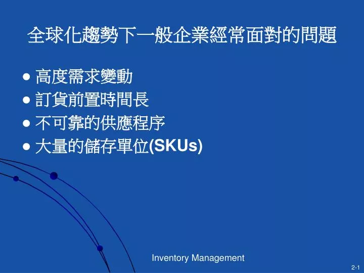
全球化趨勢下一般企業經常面對的問題 • 高度需求變動 • 訂貨前置時間長 • 不可靠的供應程序 • 大量的儲存單位(SKUs)

案例 • 三＊工業的問題…(前置時間) • 手機的產品壽命週期：200000元 (產品壽週期需求變異) • Ipad 對電子書的衝擊… (競爭需求變異) • 新機推出後一個月—IPhone跌2千；hTC跌5千；三星跌3千… • 智慧型手機可能帶來衝擊… • 電子書 • 遊戲機 • 隨身聽 • 衛星導航…

Why Is Inventory Important?1 Distribution and inventory (logistics) costs are quitesubstantial Total U.S. Manufacturing Inventories ($m): • 1992-01-31: $m 808,773 • 1996-08-31: $m 1,000,774 • 2006-05-31: $m 1,324,108 Inventory-Sales Ratio (U.S. Manufacturers): • 1992-01-01: 1.56 • 2006-05-01: 1.25

Why Is Inventory Important?2 • GM’s production and distribution network • 20,000 supplier plants • 133 parts plants • 31 assembly plants • 11,000 dealers • Freight transportation costs: $4.1 billion (60% for material shipments) • GM inventory valued at $7.4 billion (70%WIP; Rest Finished Vehicles) • Decision tool to reduce: • combined corporate cost of inventory and transportation. • 26% annual cost reduction by adjusting: • Shipment sizes (inventory policy) • Routes (transportation strategy)

Inventory • Where do we hold inventory? • Suppliers and manufacturers • warehouses and distribution centers • retailers • Types of Inventory • WIP (work in process) • raw materials • finished goods

The reasons of holding inventory • Unexpected changes in customer demand • The short life cycle of an increasing number of products. • The presence of manycompeting products in the marketplace. • Uncertainty in the quantity and quality of the supply, supplier costs and delivery times. • Delivery Lead Time, Capacity limitations • Economies of scale (transportation cost)

問題討論 • 小米3上市，對智慧型手機市場的衝擊… • 3DS上市對掌上型遊戲機市場的衝擊…

Goals: Reduce Cost, Improve Service― Example1 • By effectively managing inventory: • Wal-Mart became the largest retail company utilizing efficient inventory management • GM has reduced parts inventory and transportation costs by 26% annually

Goals: Reduce Cost, Improve Service ― Example2 • By not managing inventory successfully • In 1994, “IBM continues to struggle with shortages in their ThinkPad line” (WSJ, Oct 7, 1994) • In 1993, “Dell Computers predicts a loss; Stock plunges. Dell acknowledged that the company was sharply off in its forecast of demand, resulting in inventory write downs” (WSJ, August 1993)

Inventory Managementvs. Demand Forecasts • Uncertain demand makes demand forecast critical for inventory related decisions: • What to order? • When to order? • How much is the optimal order quantity? • Approach includes a set of techniques • INVENTORY POLICY!!

Supply Chain Factors in Inventory Policy1 • Estimation of customer demand • Replenishment lead time • The number of different products being considered • The length of the planning horizon • Service level requirements

Supply Chain Factors in Inventory Policy2 • Costs • Order cost(or setup cost): • Product cost • Transportation cost • Inventory holding cost (or inventory carrying cost): • State taxes, property taxes, and insurance on inventories • Maintenance costs • Obsolescence cost • Opportunity costs

2.2 Single Stage Inventory Control • Single supply chain stage • Variety of techniques • Economic Lot Size Model • Demand Uncertainty • Single Period Models • Initial Inventory • Multiple Order Opportunities • Continuous Review Policy • Variable Lead Times • Periodic Review Policy • Service Level Optimization

Example • Book Store Mug Sales • Demand is constant, at 20 units a week • Fixed order cost of $12.00, no lead time • Holding cost of 25%of inventory value annually • Mugs cost $1.00, sell for $5.00 • Question • How many, when to order?

2.2.1 Economic Lot Size Model (EOQ)(Ford W. Harris, 1915) Note: • No Stockouts • Order when no inventory • Order Size determines policy Inventory Order Size Avg. Inven Time Cycle Time =T

Assumptions • D items per day: Constantdemand rate • Q items per order: Order quantities are fixed, i.e., each time the warehouse places an order, it is for Q items. • K, fixed setup cost, incurred every time the warehouse places an order. • h, inventory carrying costaccrued per unit held in inventory per day that the unit is held (also known as, holding cost) • Lead time = 0 (the time that elapses between the placement of an order and its receipt) • Initial inventory = 0 • Planning horizon is long (infinite).

Deriving EOQ • Total cost at every cycle: • Cycle timeT =Q/D • Average total cost per unit time:

EOQ:Total Cost Total Cost Holding Cost Order Cost

EOQ: Optimal Order Quantity • So for our problem (Mug sales), the optimal quantity is 316

EOQ: Important Observations • Trade-off between set-up costs and holdingcosts when determining order quantity. In fact, we order so that these costs are equal per unit time • Total Cost is not particularly sensitive to the optimal order quantity

Sensitivity Analysis Total inventory cost relatively insensitive to order quantities Actual order quantity: Q Q is a multiple bof the optimal order quantity Q*. For a given b, the quantity ordered is Q = bQ*

2.2.2 The Effect of Demand Uncertainty • Most companies treat the world as if it were predictable: • Production and inventory planning are based on forecastsof demand made far in advance of the selling season • Companies are aware of demand uncertainty when they create a forecast, but they design their planningprocess as if the forecast truly represents reality • Recent technological advances have increased the level of demand uncertainty: • Short product life cycles • Increasing product variety

問題 • iPhone 5S 與 iPhone 5C的銷售量(參考iPhone 4？？) • New hTC one 的銷售量…(參考蝴蝶機…？？？)

Three principles of all forecasting techniques • The forecast is always wrong • It is difficult to match supply and demand • The longer the forecast horizon, the worse the forecast • It is even more difficult if one needs to predict customer demand for a long period of time • Aggregate forecasts are more accurate. • More difficult to predict customer demand for individual SKUs • Much easier to predict demand across all SKUs within one product family

2.2.3. Single Period Models Short lifecycle products(例如，ipad…) • One ordering opportunity only • Order quantity to be decided before demand occurs • Order Quantity > Demand => Dispose excess inventory • Order Quantity < Demand => Lose sales/profits

Single Period Models • Using historical data • identify a variety of demand scenarios • determine probability each of these scenarios will occur • Given a specific inventory policy • determine the profit associated with a particular scenario • given a specific order quantity • weight each scenario’s profit by the likelihood that it will occur • determine the average, or expected profit for a particular ordering quantity. • Order the quantity that maximizes the average profit.

Swimsuit production Example – Swimsuit production • Fashion items have short life cycles, high variety of competitors (智慧型手機？) • Swimsuit production • New designs are completed • One production opportunity • Based on past sales, knowledge of the industry, and economic conditions, the marketing department has a probabilistic forecast • The forecast averages about 13,000, but there is a chance that demand will be greater or less than this.

Demand Scenarios Example – Swimsuit production 28% 22% 18% 11% 11% 10%

Costs Example – Swimsuit production • Production cost per unit (C): $80 • Selling price per unit (S): $125 • Salvage value per unit (V): $20 • Fixed production cost (F): $100,000 • Q is production quantity

Two Scenarios Example – Swimsuit production • Scenario One: • Suppose you make 10,000 swimsuits and demand ends up being 12,000 swimsuits. • Profit = 125(10,000) - 80(10,000) - 100,000 = $350,000 • Scenario Two: • Suppose you make 10,000 swimsuits and demand ends up being 8,000 swimsuits. • Profit = 125(8,000) - 80(10,000) - 100,000 + 20(2,000) = $ 140,000

Probability of Profitability Scenarios with Production = 10,000 Units • Probability of demand being 8000 units = 11% • Probability of profit of $140,000 = 11% • Probability of demand being 12000 units = 28% • Probability of profit of $350,000 = 28% • Total profit = Weighted average of profit scenarios

Expected profit of production quantity Q1 • Di=the ith demand • Pi=the profit of production quantity Q at demand Di

Expected profit of production quantity Q2 • f(Pi)=the probability of profit P at demand DiWhen production quantity=Q • Expect Profit of Q: E(P)

Swimsuit production Solution Example – Swimsuit production • Find order quantity that maximizes weighted average profit. • Question: Will this quantity be less than, equal to, or greater thanaverage demand?

Order Quantity that Maximizes Expected Profit FIGURE 2-6: Average profit as a function of production quantity

Relationship Between Optimal Quantity and Average Demand • Compare marginal profit of selling an additional unit and marginal cost of not selling an additional unit • Marginal profit/unit = Selling Price - Variable Ordering (or, Production) Cost • Marginal cost/unit = Variable Ordering (or, Production) Cost - Salvage Value • If Marginal Profit > Marginal Cost => Optimal Quantity > Average Demand • If Marginal Profit < Marginal Cost => Optimal Quantity < Average Demand

For the Swimsuit Example • Average demand = 13,000 units. • Optimal production quantity = 12,000 units. • Marginal profit =125-80= $45 • Marginal cost = 80-20=$60. • Thus, Marginal Cost > Marginal Profit => optimal production quantity < average demand.

Risk-Reward Trade-offs • Optimal production quantity maximizes average profit is about 12,000($371000) • Producing 9,000 units or producing 16,000 units will lead to about the same average profit of $294,000. • If we had to choose between producing 9,000 units and 16,000 units, which one should we choose?

Swimsuit production Expected Profit Example – Swimsuit production 9000

Risk-Reward Tradeoffs1 89% 11% 11% -220 200 305 FIGURE 2-7: A frequency histogram of profit

Risk-Reward Tradeoffs2 • Production Quantity = 9000 units • Profit is: • either $200,000 with probability of about 11 % • or $305,000 with probability of about 89 % • Production quantity = 16,000 units. • Distribution of profit is not symmetrical. • Losses of $220,000 about 11% of the time • Profits of at least $410,000 about 50% of the time • With the same average profit, increasing the production quantity: • Increases the possible risk • Increases the possible reward

Key Insights from this Model Example – Swimsuit production • The optimal order quantity is not necessarily equal to average forecast demand • The optimal quantity depends on the relationship betweenmarginal profit and marginal cost • As order quantity increases, average profit first increases and then decreases • As production quantity increases, risk increases. In other words, the probability of large gains and of large losses increases

2.2.4. What If the Manufacturer Has an Initial Inventory? • Trade-off between: • Using on-hand inventory to meet demand and avoid paying fixed production cost: need sufficient inventory stock • Paying the fixed cost of production and not have as much inventory

Initial Inventory Solution Example – Swimsuit production 225000 FIGURE 2-8: Profit and the impact of initial inventory

Manufacturer Initial Inventory = 5,000 Example – Swimsuit production • If nothing is produced, average profit = 225,000 (from the figure) + 5,000 x 80 = 625,000 (125 5000=625000) • If the manufacturer decides to produce • Production should increase inventory from 5,000 units to 12,000 units. • Average profit = 371,000 (from the figure) + 5,000  80 = 771,000

Trade-off between Produced and not Produced Example – Swimsuit production Let X is the trade-off point

Manufacturer Initial Inventory = 10,000 Example – Swimsuit production • No need to produce anything • average profit > profit achieved if we produce to increase inventory to 12,000 units • If we produce, the most we can make on average is a profit of $371,000. • Same average profit with initial inventory of 8,245units and not producing anything. • If initial inventory < 8,245 units => produce to raise the inventory level to 12,000 units. • If initial inventory is at least 8,245 units, we should not produce anything (s, S) policy or (min, max) policy

(s, S) Policies • For some starting inventory levels, it is better to not start production • If we start, we always produce to the same level • Thus, we use an (s,S) policy. If the inventory level is below s, we produce up to S. • s is the reorder point, and S is the order-up-to level • The difference between the two levels is driven by the fixed costs associated with ordering, transportation, or manufacturing

2.2.5. Multiple Order Opportunities1 REASONS • To balanceannual inventory holding costs and annual fixed order costs. • To satisfy demand occurringduringlead time. • To protect againstuncertainty in demand.

2.2.5. Multiple Order Opportunities2 • TWO POLICIES • Continuous review policy(持續檢視政策) • inventory is reviewed continuously • an order is placed when the inventory reaches a particular level or reorder point. • inventory can be continuously reviewed (computerized inventory systems are used) • Periodic review policy(週期檢視政策) • inventory is reviewed atregular intervals • appropriate quantity is ordered after each review. • it is impossible or inconvenient to frequently review inventoryand place orders if necessary.

全球化趨勢下一般企業經常面對的問題