Download
1 / 54
540 likes | 562 Views
Pitfalls in Rock Properties and Lithology Prediction in Dolomite. John Logel Anadarko Canada Corp. Objective. To demonstrate that subtle but powerful seismic phenomenon can substantially harm your seismic data and your interpretation

E N D
Pitfalls in Rock Properties and Lithology Prediction in Dolomite John Logel Anadarko Canada Corp
Objective • To demonstrate that subtle but powerful seismic phenomenon can substantially harm your seismic data and your interpretation • TLC processing and “new” algorithms may not be enough to help • Quality control, detailed investigation of data, and proper prospecting and risk are critical.
Outline • Dolomite as the reservoir • The surprise prospect and well • The Mistie • The VSP results • The enemy (High order interbed multiples, Q) • Possible fixes and conclusions
Hydrothermal Dolomite Process Davies, et al.
Shale 2.58 g/cc 5800 P m/s 2000 S m/s 15000 AI 5200 SI 2.9 Vp/Vs 21 Gpa Bulk 7 Gpa Shear Dolomite 2.87 g/cc 7000 P m/s 3960 S m/s 20090 AI 11365 SI 1.77 Vp/Vs 95 Gpa Bulk 45 Gpa Shear Rock Properties and economic properties • Limestone • 2.71 g/cc • 6450 P m/s • 3440 S m/s • 17479 AI • 9322 SI • 1.88 Vp/Vs • 77 Gpa Bulk • 32 Gpa Shear • 50 MM.day IP • 50B – 3 TCF UR • high spacing • 10 MM/day IP • 10 B – 50 B UR • low drainage • 0 MM /day IP • 0 BCF • No more drilling AI Dolo with 10 % por = LS 6% por = Shale Vp/Vs changes less
Tuning curve for “Typical” Dolomite reservoir 0 10 20 30 40 50 amp 4 to 20 ms zone of anomolous amplitude For 45 Hz Dom freq isochron
Dolomite Zero Offset Modeling Dolomite Porosity Development Dolomite Tight Porous
Processing Highlights • Boutique TLC Processing • PSTM • 2 Passes of velocities • 2 passes and 2 different Algorithms of De-multiple (Radon and Inquisitor hyperbolic) • Controlled Amp and Phase QC • Controlled Scaling
LambdaRho - MuRho Interpretation Template Crossplot Guide LambdaRho - MuRho Interpretation Template Crossplot Guide Gas 1:1 Gas 1:1 125 125 2:1 2:1 100 100 POROUS POROUS TIGHT TIGHT DOLOMITE DOLOMITE LIMESTONE LIMESTONE .gm/cc .gm/cc Calcareous Wet Calcareous Wet Gas Gas MuRho Gpa MuRho Gpa 50 50 Shales Shales SAND SAND SHALE SHALE Clastic Clastic Shales Shales 0 0 50 100 150 200 250 50 100 150 200 250 0 0 LambdaRho GPa .gm/cc LambdaRho GPa .gm/cc 2005031a- 8 LMR Interpretation Methodology Goodway etal.
Prospect Waveform classification map Prospect And leads
Pre-drill Analysis Prospect Analogue Well lambda Analogue Mu Ratio diff Prospect
Post-Drill !! Analogue Prospect GR dt rhob GR dt rhob
Raw Synthetic tie CC= .29 Zone of Interest
Post edit Synthetic tie CC=.4 Zone of Interest
Processing Geophysicist
Other Problems, Pitfalls and Corrections • Multiples • Q (attenuation) VSP
VSP showing potential sources of Interbed multiples High velocity Low Velocity/Laminated Basin Fill Shales Inside Corridor Stack Outside Corridor Stack High Velocity Zone of Interest
VSP – Data comparison Zero (corridor) VSP stack Inside (multiple) stack seismic data Zone of Interest
VSP (downgoing colour – upgoing WVA) with Multiples Interbed multiples First arrivals Interbed multiples
Elastic Modeling Comparison Elastic Model 90 degrees Elastic Model Raw seismic Logs synthetics
Q (attenuation) • “Q” is the attenuation of frequency and the changes in phase because of it. • Shales or other “soft” material are most Q prone • Laminated material are also very Q prone • If it can be determined it can be corrected (difficult)
Wavelet extraction and response Extracted wavelet including shallow Extracted wavelet deep Theoretical response
Processed VSP and Q computation Spectral Ratio Method Drift Correction Method
Q Application correct qcomp orig
Q application and Amplitude Envelope Corrected Qcomp Orig
Final tie with synthetics validation VSP zos corrected model mult original
Questions about Multiples???? • Shouldn’t they be adequately attenuated? • Aren’t they too low of amplitude to worry about? • Aren’t they “constant”? • Shouldn’t you be able to differentiate Multiples from reservoir by a different AVO response? • Doesn’t the stack take care of it?
Questions about Multiples???? • Shouldn’t they be adequately attenuated? • Aren’t they too low of amplitude to worry about? • Aren’t they “constant”? • Shouldn’t you be able to differentiate Multiples from reservoir by a different AVO response? • Doesn’t the stack take care of it?
2D expanding models Primaries only Primaries and Multiples
2D expanding models Primaries only Primaries and Multiples
Questions about Multiples???? • Shouldn’t they be adequetely attenuated? • Aren’t they too low of amplitude to worry about? • Aren’t they “constant”? • Shouldn’t you be able to differentiate Multiples from reservoir by a different AVO response? • Doesn’t the stack take care of it?
AVO response for Dolomite Reservoir Reservoir AVO response CLASS IV
Seismic data showing horizons, multiples and VSP VSP no decon Pri & mult VSP decon Prim only Horizons Multiples
Seismic gathers showing primaries and multiples 2000 -2000
De-Multiple “Fixes” • Inquisitor Hyperbolic transform • High resolution Radon • Hybrid Radon • Inverse Scattering Subseries • Gabor decon (radial trace domain) • Wavelet Transforms • Forensic Audiology • Discrete Fourier transform • target oriented DECON • Mapping ** Discussed in this presentation
Elastic Model gather with Hyperbolic transform velocity Porosity Multiple
Principal Comps recombined Original De-Multipled
Zone specific DFT Amp Primary Dominant Freq Multiple Dominant Freq Multiple contaminated Primaries Phase
Target specific Gap decon Original Section Original De-multipled De-Multipled Section