Download
1 / 51
580 likes | 863 Views
The Diffusion Equation a nd other Similar Equations. Introduction and Preliminary Concepts Separation of Variables Sturm-Liouville Theory Fourier and Laplace Transforms. Preliminary Concepts. Linearity, Superposition and Classifications: .

E N D
The Diffusion Equation and other Similar Equations • Introduction and Preliminary Concepts • Separation of Variables • Sturm-Liouville Theory • Fourier and Laplace Transforms
Linearity, Superposition and Classifications: A partial differential operator (PDO) L is considered linear if the following is satisfied For example, therefore, PDO L is linear. Linearity, Superposition and Classification (3)
It follows that for a linear PDO the equation and heterogeneous if f is any other function. is homogeneous if The order of a PDE is determined based on the highest order derivative that is in it. For example, the inviscid Burgers’ equation below is first-order while the Korteweg-deVries (KdV) equation is third-order due to the additional term. If the linear homogeneous equation it also follows that will satisfy it. is satisfied by Linearity, Superposition and Classification (3)
In addition, PDEs can be classified based on the sign of the discriminant B2-AC using the following criteria. The heat/diffusion equation, which we will be discussing, is parabolic since, Examples of solutions of the equation are shown below. Mathematical techniques for engineers and scientists (2) Image modified from http://home.comcast.net/~sharov/PopEcol/lec12/diffus.html
Diffusion in chemical reaction* First order chemical reaction takes place on the catalyst wall of cylindrical container Find out the concentration change of A inside the container Set up PDE: D*Axx=At, or D*∂2A/∂x2 =∂A/∂t A-concentration of A D-diffusivity X=R Catalyst wall r=kA X=0 *from Chemical Engineering Kinetics (6)
Diffusion in chemical reaction First order chemical reaction takes plane on the catalyst wall Find out the concentration change of A inside the cylindrical contatiner Boundary and initial conditions: I.C t=0, A=A0 B.C1 x=0, ∂A/∂x │x=0 =0, by symmetry B.C2 x=R, D*∂A/∂x │x=R =k*A, diffusion =reaction at wall X=R Catalyst wall r=kA X=0
Diffusion in chemical reaction Run dimensionless: u=A/A0, s=x/R, τ=t/tc(=tD/R2) Then we get: tc*D/R2∂2u/∂s2 =∂u/∂τ, let tc*D/R2=1, then tc=R2/D BCs: ∂u/∂s =0 at s=0 ∂u/∂s =kR/D*u=φu, φ=kR/D at s=1 X=R Catalyst wall r=kA X=0
Diffusion in chemical reaction Assume: u=F(s)*G(τ) G(τ)*dF2/ds2=F(s)*dG(τ)/ds, 1/F(s)*dF2/ds2=1/G(τ)*dG(τ)/ds=-λn2 Solve 1/G(τ)*dG(τ)/ds=-λn2 we get: dG(τ)=exp(-λn2τ) For 1/F(s)*dF2/ds2=-λn2 assume F(s)=∑(Ansinλns+ Bncosλns) X=R Catalyst wall r=kA X=0
Diffusion in chemical reaction Use BC1: ∂u/∂s =0 at s=0 ∂u/∂s=G(τ)*dF/ds=0 ∑(Anλncosλn*0- Bnλnsinλn*0)=0 An=0 F(s)= ∑Bncosλns Use BC2: ∂u/∂s =φu at s=1 -Bnλnsinλn=φBncosλn -λntanλn=φ, λncan be solved X=R Catalyst wall r=kA X=0
Diffusion in chemical reaction u(s, τ) =∑exp(-λn2 τ)Bncosλns How to get Bn? τ =0, u(s,0)=1= ∑1*Bncosλns Use orthogonality principle ∫01 *cos(λns)ds =Bn∫01cos2(λns)ds Bn =∫01 cos(λns)ds/∫01cos2(λns)ds Bn =4sin(λn )/(2λn+sin2λn) X=R Catalyst wall r=kA X=0
What are Strum-Liouville Problems? • Second order, homogenous, linear differential equation with boundary conditions. • Solutions to such problems contain an infinite set of eigenvalues with corresponding eigenfunction solutions
A simple example: Problem from Introduction to Differential Equations (7)
How is this useful for Separation of Variables? • Many differential equations are in the form of the Sturm-Liouville problem. • Sturm-Liouville analysis can help determine integration constants for equations with an infinite number of terms (eigenfunctions).
A more complex example: Problem from Heat Conduction (8)
The boundary conditions are such that Figure from Heat Conduction (8)
Other considerations considerations: • Other types of problems • Wave equation, diffusion equation… • Other types of boundaries: • Fixed, Periodic, Moving • Handled same as in regular Sturm-Liouville Problem
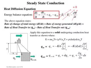
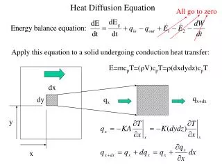
Diffusion Equation: The energy balance over the infinitesimal volume of a rod shown in the figure is as follows where, m=AΔxσc. Dividing the full equation by AΔxσc and taking the limit as x goes to 0 yields Variables: Heat Conduction and the Heat Equation (5) Image modified from http://www.ceb.cam.ac.uk/pages/finite-element-simulations.html
Initial/Boundary Conditions: For all subsequent calculations we assume that diffusion in the rod is one-dimensional and thus set H and and v to zero. The initial condition is simply a set function for u(x,t) over the length of the rod at t=0 and is written thus, The boundary condition can fall into one of three categories. Dirichlet boundary condition: Meaning that the left end of the bar is kept at a set temperature. Neumann boundary condition: This boundary condition specifies the heat flow out of the rod. Particularly, setting means insulating the left end of the rod. Fundamental Solutions (4)
Initial/Boundary Conditions (cont`d): Robin boundary condition: Starting with Newton’s Law of Cooling where, us and uf are temperatures of the solid and fluid respectively. It then follows that, Heat Conduction and the Heat Equation (5)
For non-periodic functions [f(x)] the heat equation can be solved using Fourier exponential transform and a known Gaussian function g(x,t) the steps follow….. Heat Conduction of an Infinite Rod (Fourier Transforms) Mathematical techniques for engineers and scientists (2)
The Fourier exponential transform can be written as Using the above definition we can write The heat equation can then be rewritten as We can solve for U using the initial condition to yield Thus, ……(1) Mathematical techniques for engineers and scientists (2)
Special Case 1: The simplest solution to the heat equation is for Assuming that all terms except a are constant the function can be integrated to yield Thus, for the limiting case of f(x) = constant the heat will also equal that constant. Advanced engineering mathematics (9)
Special Case 2: In this case, assume the initial condition is as follows Using these initial conditions the heat equation can be solved to yield since the integral can then be rewritten as Beny Neta Presentation (1)
From the chart we can see the function “smoothing” out at large values of t. This is due to the behavior of the error function, erf(∞)=1 and erf(~0)=0. Thus, for positive values of x at small times u(x,t) approaches F and at large times u(x,t) approaches F/2. For negative values of x the negative sign can be taken outside of the error function so the value of the error function is subtracted from 1. Thus at small times u(x,t) approaches 0 and at large times u(x,t) approaches F/2.
Typical Behavior The following curves are of temperature collected at different times. From the plots a “smoothing” effect can again be seen as the temperature along entire length of the rod approaches an equilibrium value. Images taken from http://en.wikipedia.org/wiki/File:Heatequation_exampleB.gif
Special Case 3: Similar to the error function the integral of equation (1) can be rewritten as the kernel K to t1 and the function becomes…. t2 x From the graph you can see that similar “smoothing” process occurs for the Kernel as for the temperature profile. It is also important to note that the Kernel is a response function to an initial temperature function described by the delta function figure modified from: http://mobjectivist.blogspot.com/2010_06_01_archive.html
Heat Conduction of a Semi-Infinite Rod (Laplace Transforms) For non-periodic functions [f(x)] the heat equation can be solved in the semi-infinite domain using Laplace exponential transform the steps follow….. Mathematical techniques for engineers and scientists (2)
Using the inverse Laplace transform U(x,p) becomes, Then using the convolution theorem u(x,t) becomes, ………(2) Mathematical techniques for engineers and scientists (2)
The Laplace exponential transform can be written as Using the above definition we can write The heat equation can then be rewritten as We can solve for U using the boundary condition to yield Mathematical techniques for engineers and scientists (2)
Special Case : The simplest solution to the heat equation is for By setting we can solve for and Thus equation (2) becomes or otherwise Advanced engineering mathematics (9)
For F=50 and α=1 u(x,t) is plotted below From the chart we can see a similar “smoothing” process as in the case of the infinite domain at large values of t. Again, erf(∞)=1 and erf(~0)=0. Thus at small times u(x,t) approaches F and at large times u(x,t) approaches 0.